
Table 1
Construction of the locked-in status variable (the new values in brackets).
| Workplace non-preference | Perceived Employability | |
|---|---|---|
| Low | High | |
| 1 = Preferred job | NLI (1) | NLI (1) |
| 2 = Non-preferred workplace, but OK for now | RLI (2) | NLI (1) |
| 3 = Non-preferred workplace | LI (3) | NLI (1) |
[i] LI: being locked in, RLI: at risk of becoming locked in, NLI: not locked in.
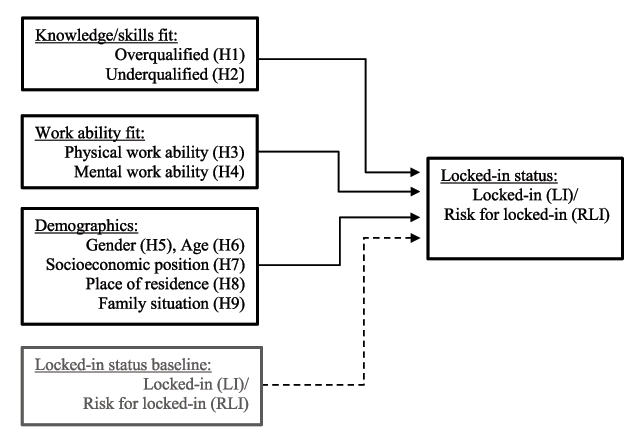
Figure 1
The study hypotheses. For the cross-sectional hypotheses, both independent and dependent variables are measured at Time 1. For longitudinal hypotheses, the independent variables are measured at Time 1, whereas the dependent variable is measured at Time 2. Note that locked-in status baseline (Time 1) only is controlled for in the analyses of longitudinal relations (the dashed line).
Table 2
Multinomial logistic regressions. Matching factors between work and individuals. Odds ratios and 95% confidence intervals.
| Locked-in status T1 (Cross-sectional) | Locked-in status T2 (Longitudinal, including locked-in status baseline) | |||||||||
|---|---|---|---|---|---|---|---|---|---|---|
| RLI | LI | % | RLI | LI | % | |||||
| Odds ratios | 95% CI | Odds ratios | 95% CI | Odds ratios | 95% CI | Odds ratios | 95% CI | |||
| Knowledge/skills fit | ||||||||||
| Overqualified | 1.67*** | [1.43, 1.93] | 3.18*** | [2.48, 4.07] | 21.6 | 1.01 | [0.80, 1.26] | 1.80** | [1.25, 2.58] | 21.1 |
| Underqualified | 1.22* | [1.03, 1.45] | 1.26 | [0.90, 1.75] | 16.4 | 1.03 | [0.80, 1.32] | 1.22 | [0.77, 1.91] | 16.9 |
| Well-matched (ref.) | – | – | – | – | 62.0 | – | – | – | – | 62.0 |
| Work ability fit | ||||||||||
| Poor physical work ability1 | 1.33*** | [1.18, 1.50] | 1.10 | [0.89, 1.37] | – | 1.15 | [0.96, 1.38] | 1.38* | [1.04, 1.84] | – |
| Poor mental work ability1 | 1.50*** | [1.30, 1.73] | 2.72*** | [2.24, 3.29] | – | 1.39** | [1.13, 1.72] | 1.40* | [1.01, 1.93] | – |
| Locked-in status baseline | ||||||||||
| LI | 5.2 | 6.96*** | [4.79, 10.13] | 29.43*** | [18.94, 45.74] | 4.8 | ||||
| RLI | 19.8 | 8.13*** | [6.69, 9.90] | 7.01*** | [4.83, 10.18] | 18.5 | ||||
| NLI (ref) | 75.1 | – | – | – | – | 76.7 | ||||
| N | 6449 | 3898 | ||||||||
| Nagelkerke R2 | .055 | .245 | ||||||||
[i] Reference profile: Non-locked-in at Time 2. Locked-in status distribution at Time 2 (LI: 4.7%, RLI: 17.2%, NLI: 78.1%).
* p < 0.05; ** p < 0.01; *** p < 0.001; † p < 0.10.
All independent variables at T1 (2014).
Table 3
Multinomial logistic regressions. Demographic factors. Odds ratios and 95% confidence intervals.
| Locked-in status T1 (Cross-sectional) | Locked-in status T2 (Longitudinal, including locked-in status baseline) | |||||||||
|---|---|---|---|---|---|---|---|---|---|---|
| RLI | LI | % | RLI | LI | % | |||||
| Odds ratios | 95% CI | Odds ratios | 95% CI | Odds ratios | 95% CI | Odds ratios | 95% CI | |||
| Gender (female) | 0.94 | [0.83, 1.08] | 0.80† | [0.63, 1.02] | 57.5 | 0.86 | [0.71, 1.04] | 0.62** | [0.44, 0.87] | 57.7 |
| Age | ||||||||||
| Less than 35 years | 0.95 | [0.75, 1.21] | 0.77 | [0.49, 1.23] | 9.6 | 0.92 | [0.62, 1.35] | 0.55 | [0.26, 1.20] | 7.8 |
| More than 49 years | 1.01 | [0.87, 1.18] | 0.99 | [0.75, 1.31] | 51.8 | 1.00 | [0.80, 1.24] | 0.93 | [0.63, 1.36] | 53.3 |
| 35–49 years (ref.) | – | – | – | – | 38.6 | – | – | – | – | 38.8 |
| Socioeconomic position | ||||||||||
| Unskilled manual | 1.61*** | [1.32, 1.95] | 1.61** | [1.14, 2.28] | 11.9 | 1.27 | [0.93, 1.73] | 1.14 | [0.64, 2.03] | 9.8 |
| Skilled manual | 1.02 | [0.84, 1.24] | 0.87 | [0.60, 1.27] | 14.4 | 1.01 | [0.75, 1.35] | 0.92 | [0.52, 1.61] | 13.1 |
| Assistant non-manual | 1.56*** | [1.29, 1.89] | 1.90*** | [1.38, 2.61] | 12.6 | 1.50** | [1.12, 2.01] | 2.77*** | [1.78, 4.32] | 11.0 |
| Medium/higher non-manual (ref.) | – | – | – | – | 61.1 | – | – | – | 66.1 | |
| Place of Residence | ||||||||||
| Urban areas | 0.78** | [0.66, 0.93] | 1.10 | [0.80, 1.51] | 34.4 | 0.74* | [0.57, 0.95] | 1.31 | [0.82, 2.09] | 34.7 |
| Semi-urban areas | 0.98 | [0.83, 1.15] | 1.17 | [0.86, 1.58] | 40.0 | 0.81† | [0.64, 1.02] | 1.14 | [0.72, 1.79] | 40.2 |
| Sparsely populated areas (ref.) | – | – | – | 25.6 | – | – | – | – | 25.1 | |
| Family situation | ||||||||||
| Marital status (married/cohabitant) | 0.85* | [0.72, 1.00] | 0.82 | [0.62, 1.10] | 79.7 | 0.94 | [0.74, 1.20] | 0.79 | [0.52, 1.20] | 80.1 |
| Parental status (children at home) | 1.16† | [1.00, 1.34] | 0.96 | [0.74, 1.26] | 51.0 | 1.18 | [0.95, 1.46] | 1.01 | [0.69, 1.49] | 52.4 |
| Locked-in status baseline | ||||||||||
| LI | 5.1 | 7.63*** | [5.19, 11.23] | 38.84*** | [24.63, 61.23] | 4.8 | ||||
| RLI | 19.5 | 8.33*** | [6.79, 10.20] | 7.82*** | [5.28, 11.60] | 18.3 | ||||
| NLI (ref) | 75.4 | – | – | – | – | 76.9 | ||||
| N | 5984 | 3633 | ||||||||
| Nagelkerke R2 | .018 | .256 | ||||||||
[i] Reference profile: Non-locked-in at Time 2. Locked-in status distribution at Time 2 (LI: 4.6%, RLI: 17.2%, NLI: 78.2%).
* p < 0.05; ** p < 0.01; *** p < 0.001; †p < 0.10.
All independent variables at T1 (2014).