Precise assessment of organ volume or volumetric changes holds importance in diagnostics, prognostic forecasting, and tailoring treatment for patients. An array of imaging techniques is used to evaluate gallbladder volumes and motility, including magnetic resonance cholangiopancreatography (MRCP), cholecystography, cholescintigraphy, and transabdominal ultrasound(1,2,3,4,5,6). However, none of these methods has achieved widespread use.
Traditional two-dimensional (2D) ultrasound has been the cornerstone in gallbladder evaluation for decades and remains the first-line imaging modality for examining the gallbladder and biliary system in patients with suspected biliary diseases, such as cholecystitis, gallbladder polyps, and cholelithiasis(7,8). Compared with other imaging modalities, ultrasonography offers the advantage of on-the-spot real-time examination by clinicians, facilitating immediate diagnosis. However, 2D ultrasound may have limitations in gallbladder volume estimation. The most common method for estimating volume based on 2D ultrasound, known as the ellipsoid method, assumes that the gallbladder conforms to an ellipsoid shape. This assumption may introduce inaccuracies due to the gallbladder’s inherently non-ellipsoid morphology. The sum-of-cylinders method derived from 2D ultrasound has been suggested for more accurate volume estimation(9). However, this method is more time-consuming and not significantly more accurate compared to other 2D ultrasound-based methods, including the ellipsoid method(10,11). Another 2D-based approach is planimetry(12,13).
The geometric assumptions of 2D ultrasound can be avoided by using 3D ultrasound methods. The benefits of 3D have been shown in volumetric studies of several organs, including the stomach, kidneys, prostate, and urinary bladder(14,15,16,17). Several methods have been developed, and ultrasound system manufacturers offer both automatic, semi-automatic, and manual tracing options depending on the organ being evaluated. Previous studies have shown that 3D ultrasound of the gallbladder is both reliable and feasible, with accuracy similar to, or better than, that of 2D ultrasound, even if the operator is unskilled in ultrasound imaging(10,11,18). Moreover, 3D ultrasound volumetry correlates well with measurements obtained from cholecystograms(19).
The present study was designed to evaluate whether the conventional ellipsoid formula applied to 2D ultrasound images provides a sufficiently accurate estimate of organ volume compared with 3D ultrasound volumetry. The gallbladder was selected as a model organ because it is easily visualized, exhibits both ellipsoid and irregular morphologies, and undergoes reproducible volume changes during fasting and following meal intake, making it well suited for methodological comparison.
In this study, we aimed to compare the precision and feasibility of gallbladder volume measurements using 2D and 3D transabdominal ultrasound in an adult patient cohort.
In this cross-sectional, observational study, adult participants were enrolled between May 2019 and September 2021 at Haukeland University Hospital in Bergen, Norway. Although participants were originally included as part of a broader project investigating gastrointestinal autonomic function in type 2 diabetes mellitus, the current substudy pooled all participants irrespective of diabetic status. The aim of this analysis was strictly methodological—comparing 2D and 3D ultrasound techniques for gallbladder volume estimation rather than evaluating disease-related differences.
The study was conducted in accordance with the Declaration of Helsinki and approved by the Regional Committees for Medical and Health Research Ethics, Western Norway (reference number 2018/1790). All participants provided written informed consent prior to inclusion.
Upon inclusion, participant characteristics were recorded, including age, sex, body mass index (BMI), and smoking status.
Prior to ultrasound examinations, participants had fasted overnight (i.e. for a minimum of eight hours). Scans were performed at specific time intervals (15 and 5 min) before and (10, 20, 30, 40, 50, 60, 70, 80, 90, 105, and 120 min) after ingestion of a standardized meal consisting of a nutritional drink. The drink (200 mL Fresubin, wild berries flavor, Fresenius Kabi, Germany) contained a total of 400 kcal, 20 g protein, 15.6 g fat, and 45 g carbohydrates. A graphical representation of the timeline is provided in Supplemental Fig. S1.
The examinations were performed using a GE Logiq E9 ultrasound system (GE Healthcare, Chicago, IL, USA). The 2D and 3D ultrasound images were acquired with a GE C1-5-D probe (1–5 MHz, curvilinear) and a GE RAB2-5-D probe (2–5 MHz, curvilinear), respectively. Participants were examined in the supine position. The probe was positioned subcostally on the right upper abdomen when feasible, or intercostally when subcostal imaging did not provide sufficient visualization. In addition to probe placement, participant positioning and breath-holding were used to improve visualization. At each acquisition interval, the gallbladder was sequentially scanned twice in 2D followed by twice in 3D. The four resulting datasets were denoted 2D(a), 2D(b), 3D(a), and 3D(b). Between participants, the scanning order (2D or 3D first) was alternated randomly to reduce systematic bias.
Each dataset was acquired during a breath-hold to minimize motion artefacts. Because the gallbladder is anatomically distant from the heart, cardiac motion was not considered to influence volume assessment, and ECG gating was therefore not applied.
The 2D examinations were performed using the following settings: frequency 4.0 MHz, dynamic range 66, and frame rate 26 frames per second. The gallbladder was measured in three dimensions: length (L) in the longitudinal plane, and width (W) and height (H) perpendicular to it in the cross-sectional plane. With the assumption of the gallbladder having an ellipsoid form, the volume V2D was calculated by using the following equation: V2D = (π/6) × L × W × H
The 3D volume datasets were obtained during a fully automated acquisition lasting approximately one second or less. The GE Healthcare Virtual Organ Computer-Aided Analysis (VOCAL) tool reconstructed a predefined number of slices (typically six, but up to 20 for irregularly shaped gallbladders) from each single 3D scan. Thus, the difference between six and 20 slices reflects only the number of processed planes, not the duration of data capture; therefore, the timing between slices was negligible. VOCAL offers both semi-automatic and manual tracing options; in this study, manual tracings were performed. The position and size of the region of interest (ROI) were adjusted to include the entire gallbladder in the longitudinal plane. All measurements were acquired during breath-hold. Depending on gallbladder morphology, rotational step angles of 30°, 15°, or 9° (corresponding to six, 12, or 20 slices) were used to ensure adequate spatial sampling of the organ volume. The relatively short acquisition time (≤5 s per scan) rendered the effect of temporal variation negligible. Finally, the system calculated the volume (cm3) of the gallbladder based on the traced areas. The full temporal sequence of data collection, including pre- and post-meal imaging time points, is illustrated in Supplemental Fig. S1.
Statistical analyses were performed, and graphs were generated using R version 4.3.3 in RStudio Desktop 2023.12.1+402 (Posit PBC, Boston, MA, USA) and Prism 10 for macOS (GraphPad Software, LLC., v10.1.1). The values of characteristics are presented as means with standard deviation (SD) or median with interquartile range (IQR), as appropriate. Means were compared using Dunn’s multiple comparisons test. Normality was tested using a combination of histograms, quantile-quantile (Q-Q) plots, Shapiro-Wilk test, Anderson-Darling test, Kolmogorov-Smirnov test, and D’Agostino & Pearson test. Outliers were detected using the ROUT method(20). Time points with incomplete datasets, i.e., where at least one of the four measurements for a given time point for a participant was missing, were excluded from further calculations. All other complete time points from the same participant were retained. Agreement between gallbladder volumes was tested using a single-rater, two-way random-effect model intraclass correlation coefficient(21). Agreement was visualized using Bland-Altman plots, with limits of agreement set to 95% confidence interval (CI). For correlation analyses, Pearson’s correlation coefficient was used, as the data were approximately normally distributed and the relationships between variables were linear. For multiple comparisons, Holm-Šidák’s correction was used. Statistical significance was set at p <0.05.
Sixty-six participants were enrolled. Four participants were excluded, two due to inadequate visualization of the gallbladder and two due to previous cholecystectomy. Among the 62 included participants, 34 had type 2 diabetes mellitus and 28 were non-diabetic. The study participants had a mean age of 69 years and a median BMI of 24 kg/m2 (Tab. 1).
Clinical characteristics of the included subjects
| Variables | Values | Range (Min–Max) |
|---|---|---|
| N | 62 | N/A |
| Sex, males (%) | 31 (50.0) | N/A |
| Age, mean (SD) in years | 69.1 (6.6) | 52.0–84.0 |
| BMI, median (IQR) in kg/m2 | 24.3 (22.9–28.6) | 18.5–33.3 |
| Smoking status, % present / past / never | 6.5/33.9/59.7 | N/A |
N/A – not applicable; SD – standard deviation; BMI – body mass index; IQR – interquartile range
A rotational step angle of 30° was used in all participants except two. In these two participants, rotational step angles of 15° and 9° were used.
Among the volume calculations, a total of 92 out of 2,440 data-points (3.75%) were classified as outliers (Supplemental Fig. S2).
After excluding outliers and time points with missing datapoints, 582 unique time points and 2,328 data points remained for analysis. No conclusions of the study were altered by excluding the outliers, although analyses without outliers yielded reduced standard deviations and narrower 95% CIs. Normality testing indicated that the 2D data had a higher probability of being log-normally distributed, while the 3D data were normally distributed. To facilitate comparison between 2D and 3D data, the data were assumed to be normally distributed in subsequent analyses.
The distribution of gallbladder volumes across the 2D and 3D datasets is illustrated in Fig. 1. The mean volumes of the 2D datasets were 23.8 cm3 (SD 20.0 cm3) for 2D(a) and 23.8 cm3 (SD 19.7 cm3) for 2D(b). For 3D, the mean volumes were 21.6 cm3 (SD 22.7 cm3) for 3D(a) and 21.6 cm3 (SD 22.7 cm3) for 3D(b).
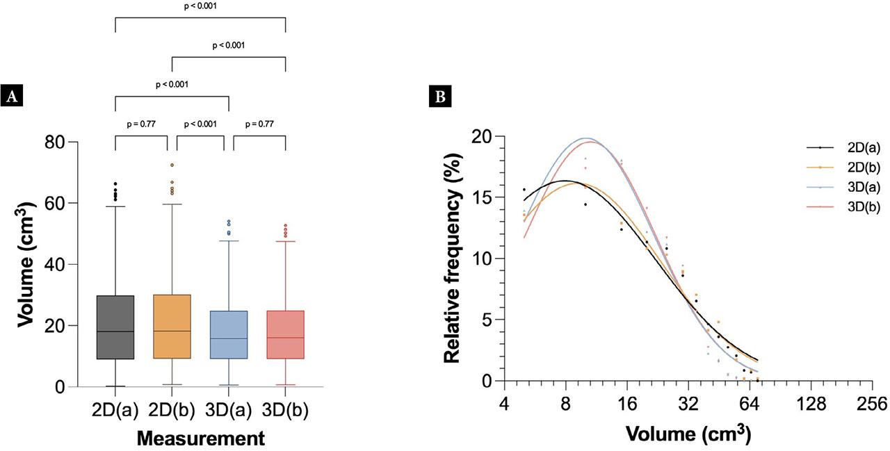
Tukey plot (A) and histogram (B) showing the distribution of gallbladder volumes for each dataset after outlier removal. A one-way ANOVA (Holm-Šidák’s multiple comparison) showed that only the 2D vs 3D datasets were significantly different (p <0.001), whereas the comparisons of 2D(a) vs 2D(b) or 3D(a) vs 3D(b) were not significantly different
The results showed a similar size distribution between the two 2D datasets and the two 3D datasets, but a significant difference between 2D and 3D measurements. The differences between 2D and 3D were significant across all datasets. The histogram shows that smaller volumes (<30 cm3) were underestimated using 2D, whereas larger volumes (>30 cm3) were slightly overestimated using 2D compared to 3D.
When comparing the sequential 2D scans, the ICC was 0.94 (p <0.001, 95% CI 0.94–0.95). The Pearson’s correlation coefficient was 0.94 (p <0.001, 95% CI 0.93–0.95). Similarly, when comparing the 3D sequential scans, a high level of agreement was found, with the ICC between the two measurements being 0.96 (p <0.001, 95% CI 0.96–0.97). The Pearson’s correlation coefficient was 0.96 (p <0.001, 95% CI 0.96–0.97). Correlation plots illustrating the differences between the sequential scans in 2D and 3D can be found in Fig. 2A,B.
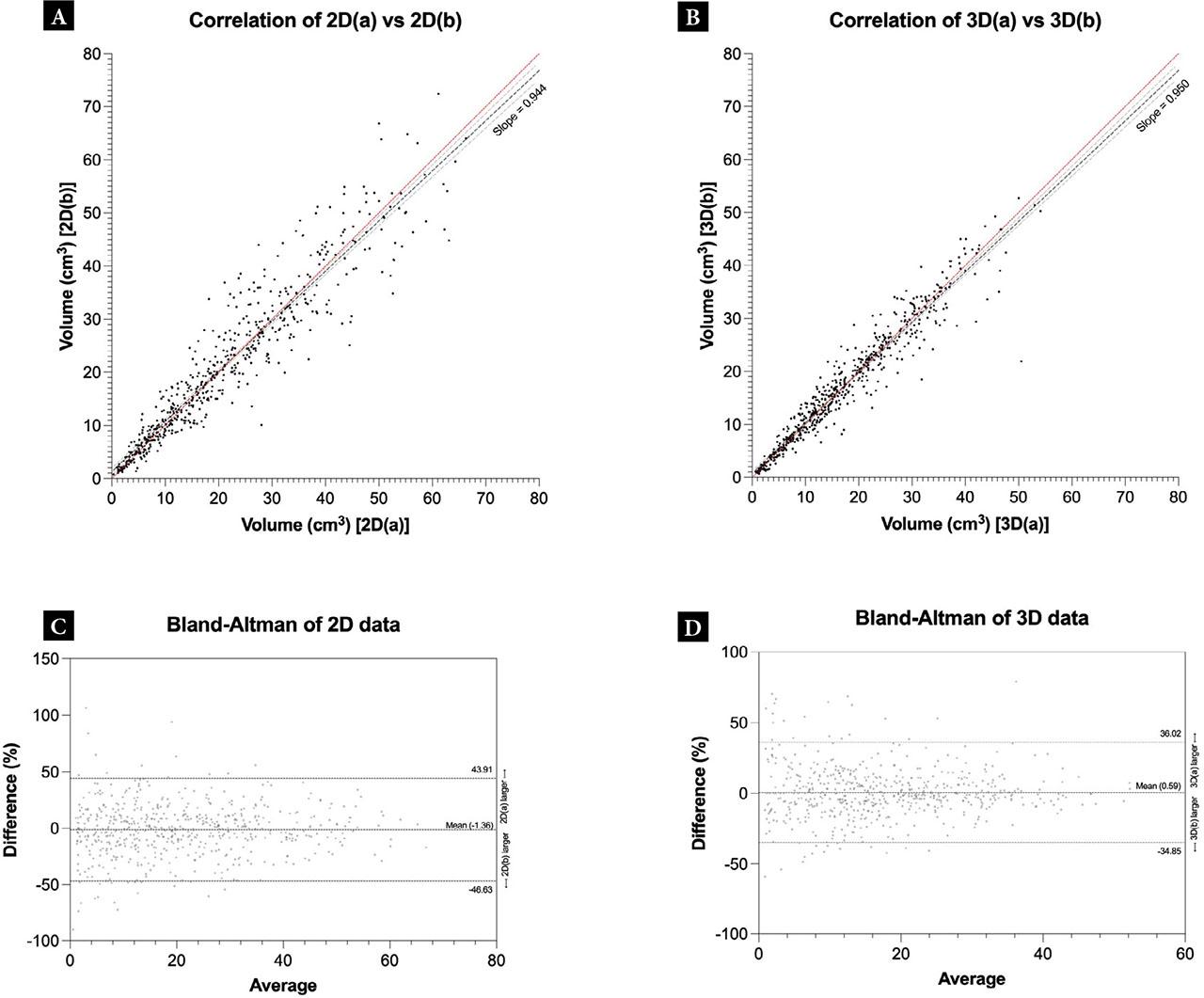
Comparison of intra-observer volumes within the 2D and 3D datasets. A, B. Correlation plots showing the association between gallbladder volume measurements from two sequential scans for 2D and 3D, respectively. The red line indicates the line of identity. The dashed lines show a linear regression, with the light dashed lines representing the 95% confidence interval of the linear regression. B, C. Bland-Altman plots showing the differences vs. average between gallbladder volume measurements of two sequential scans for 2D and 3D, respectively. The dashed lines represent the upper and lower limits of agreement or the mean value (bias)
Bland-Altman analysis evaluating bias and agreement showed that, in the 2D dataset, the mean was −1.36 ± 23.10%, with 95% limits of agreement of −46.63–43.91. In the 3D dataset, the mean was 0.58 ± 18.08%, with 95% limits of agreement of −34.85–36.02. The Bland-Altman plots are shown in Fig. 2C,D.
For the comparison of 2D and 3D measurements, the mean volume of two sequential scans was used. Fig. 3A shows the combined distribution of measured volumes. The 2D measurements had a mean of 21.0±14.4 cm3 (95% CI 19.81–22.16), and the 3D measurements had a mean of 17.7 ± 10.9 cm3 (95% CI 16.84–18.62). A Kolmogorov-Smirnov test resulted in p <0.001. The ICC between 2D and 3D was 0.85 (95% CI 0.74–0.91, p <0.001).
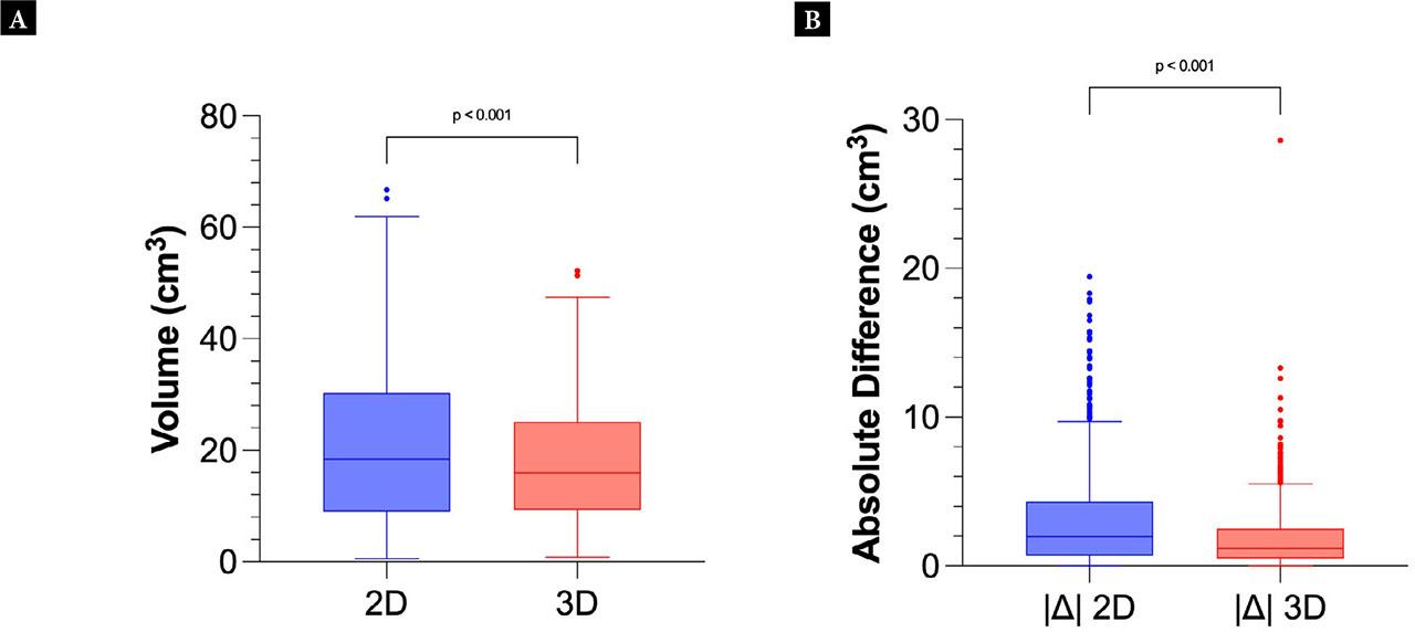
Tukey plot of the mean 2D volumes vs 3D volumes (A). Tukey plot showing the absolute differences |Δ| within the sequential 2D or 3D volume calculations (B)
The absolute differences of volumes from the sequential 2D and 3D scans were calculated and presented in Fig. 3B. This allowed visualization of the difference within each data capture method in intra-observer analysis. A two-tailed Welch’s t-test gave p <0.001, confirming the hypothesis that intra-observer variability was significantly different between the 2D and 3D methods. When computing the volume using 2D ultrasound, the mean difference in the intra-observer analysis was 3.3 cm3, whereas in 3D the mean difference was 1.9 cm3.
Figure 4 shows the correlation plot and the Bland-Altman plot comparing 2D and 3D, respectively. The Pearson’s correlation coefficient between 2D and 3D was 0.92 (95% CI 0.90–0.93, p <0.001) whereas the Bland-Altman analysis shows a mean of 11.54 ± 34.50%, with 95% limits of agreement from −56.07 to 79.16.
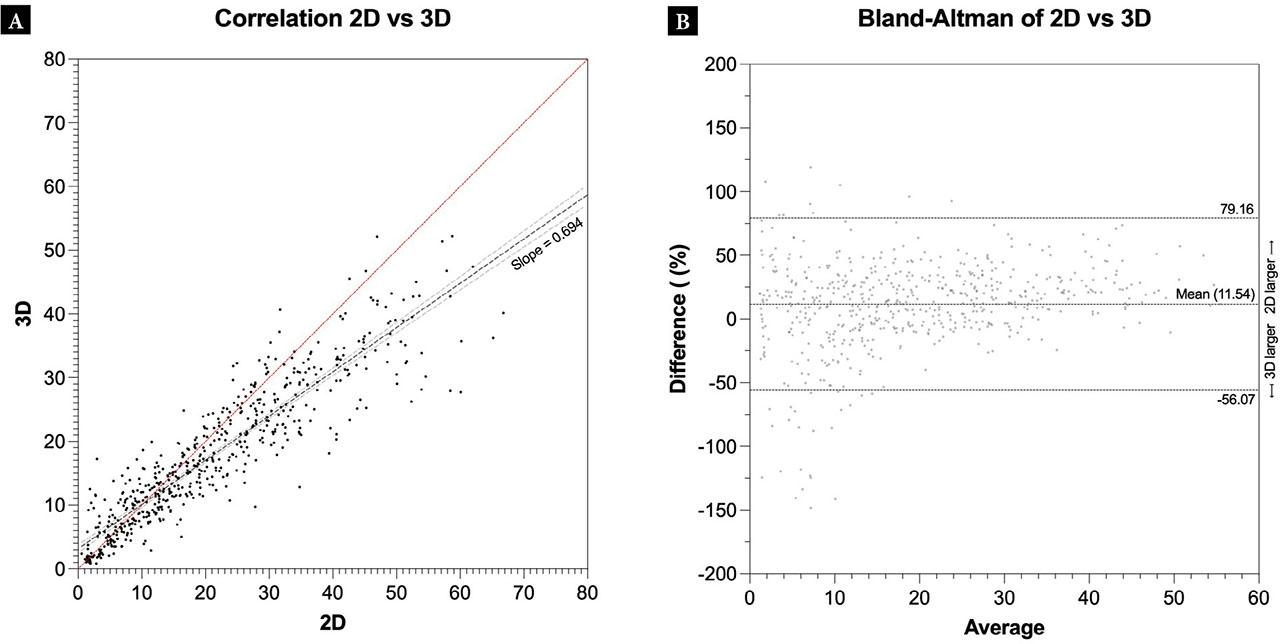
Correlation plots showing the differences (cm3) between gallbladder volumes from 2D and 3D scans. The dashed lines show a linear regression, with the light dashed lines representing the 95% confidence interval of the linear regression (A). Bland-Altman plots showing the differences (%) in gallbladder volumes for 2D vs 3D. The difference is calculated as 2D minus 3D. The dashed lines represent the limits of agreement (B)
This cross-sectional study on 62 participants aimed to compare post-prandial gallbladder volumes acquired by 2D and 3D ultrasound. A significant difference was found between 2D and 3D ultrasound volumes, with agreement between 2D and 3D volumes being lower than the intra-observer agreement for either method. The mean differences between sequential measurements were smaller in 3D compared to 2D, indicating higher precision when using 3D ultrasound to measure gallbladder volume.
After excluding outliers, the intra-observer correlation was lower for 2D volumes than for 3D volumes. This can be attributed to the narrower distribution of data in the 3D dataset vs. the 2D dataset (see Fig. 1, Fig. 2, Fig. 3, and Fig. 4). Furthermore, the Bland-Altman plots showed a smaller bias (i.e., a mean closer to zero), smaller standard deviation, and smaller 95% limits of agreement for 3D. Given this difference in distribution, when comparing 2D to 3D, a noticeable difference was visualized. Specifically, at lower volumes, the 3D measurements were larger than the 2D measurements, and at volumes above approximately 30 cm3, the 2D measurements were larger than the 3D measurements. This can be seen in Fig. 1 and Fig. 4, and similar findings have been reported by other authors(22). This discrepancy at larger volumes may be due to the non-ellipsoid shape of the gallbladder. Specifically, selecting the largest diameters assumes that at no point does the gallbladder boundary deviate significantly from the ellipsoid boundary. Supplemental Fig. S3 illustrates examples where the 2D method would include non-gallbladder volumes into the calculation, resulting in a 2D calculation overestimation; or miss gallbladder volume, resulting in a 2D calculation underestimation. At smaller volumes, the impact of this error would not result in a significant difference in volume, as the discrepancy itself would also remain proportionally small. In contrast, at larger volumes, incorrect boundary definitions result in larger errors. This hypothesis is consistent with what is observed in Fig. 1 and Fig. 4. In contrast, at smaller true volumes, while an error may not have a major numerical value difference, the percentage difference would be substantial. This hypothesis is supported by Fig. 2.
The feasibility of 2D and 3D ultrasound for the measurement of gallbladder volumes have been shown by this and previous studies(11,18,19,22,23). Ultrasound methods, participant selection, and additional modality or in vitro involvement vary between studies. In our study, we found high and similar intra-observer agreements for 2D and 3D ultrasound, but somewhat lower agreement when comparing the two methods. Based on the reduced dispersion of 3D volume data vs 2D volume data and the ability to measure volumes more accurately using 3D segmentation, our results indicate that gallbladder volume estimation is more precise using 3D ultrasound versus 2D ultrasound. Literature supports that 3D ultrasound-based volume estimation provides results closer to the true volume(22,23) and is reproducible even with less skilled operators(18). However, 2D-based volume estimation is less time-consuming, and it has been suggested that 2D may be easier to perform in patients with gallstones, as 2D ultrasound is less reliant on complete visualization of the borders of the gallbladder wall(22).
The primary limitation of 3D ultrasound is the time-consuming post-processing required for manual tracing. Numerous commercially available ultrasound system already perform automatic and Artificial Intelligence-assisted volume estimation of bladders (e.g., Butterfly Network, Clarius, Verathon, Echonous, and more). Such systems perform real-time 3D volume calculations using 2D ultrasound arrays. Given the visual similarity between the urinary bladder and gallbladder, it can be assumed that developing a similar automated 3D gallbladder volume estimation may be feasible, combining the cost benefits of 2D ultrasound and the performance benefits of 3D ultrasound. For now, the choice between 2D and 3D may be guided by local availability, examiner skill, patient characteristics, and the need for high precision.
In a clinical setting, measuring gallbladder emptying using 3D ultrasound may be indicated in individuals with biliary symptoms despite the absence of gallstones. Such patients may be evaluated for functional gallbladder disorders, such as biliary dyskinesia and chronic acalculous cholecystitis(23,24). Impaired gallbladder emptying has also been suggested as a consequence of autonomic neuropathy in patients with diabetes mellitus(25,26). As such, 3D ultrasound could be evaluated as a tool for assessing gastrointestinal autonomic neuropathy in diabetes. However, further studies are needed to evaluate the role of 3D ultrasound evaluations of gallbladder emptying in these conditions.
The lack of true gallbladder volumes limits the understanding of differences in volumes obtained by 2D and 3D ultrasound and the conclusions that can be drawn from this study. True volumes could have been obtained by simultaneously performing MRI, but this was not feasible within our study protocol. However, several previous studies(9,10,11,19,22,23) have demonstrated that ultrasound is reliable by comparing it with other imaging modalities and ultrasound examinations of phantoms.
There were significant differences between gallbladder volumes measured by 2D and 3D ultrasound imaging. The deviation between the two modalities increased with larger gallbladder volumes. The precision of 2D measurements was reduced compared to that of 3D. However, whether the small differences between 2D and 3D ultrasound may have impact on diagnostic performance remains unknown and warrants further investigation.