
Table 1.
Ethnic composition and its changes in Latvia, 2000–2019 (Central Statistical Bureau of Latvia).
| Ethnic group | Total population 2019 | Population change 2000–2019 | Mean age | ||||
|---|---|---|---|---|---|---|---|
| number | % of total | % of ethnic minorities | number | % | 2000 | 2019 | |
| Latvians | 1,196,251 | 62.3 | – | −174,305 | −12.7 | 36.8 | 40.4 |
| Russians | 478,578 | 24.9 | 66.2 | −224,539 | −31.9 | 39.5 | 47.4 |
| Belarusians | 61,418 | 3.2 | 8.5 | −35,719 | −36.8 | 44.7 | 55.4 |
| Ukrainians | 43,062 | 2.2 | 6.0 | −20,572 | −32.3 | 41.9 | 52.5 |
| Poles | 38,818 | 2.0 | 5.4 | −20,680 | −34.8 | 42.0 | 50.9 |
| Lithuanians | 22,340 | 1.2 | 3.1 | −11,085 | −33.1 | 42.3 | 51.0 |
| Other | 79,040 | 4.1 | 10.9 | +29,345 | +59.0 | 36.2 | 24.0 |
| Total | 1,919,507 | −457,555 | −19.2 | 38.2 | 42.5 | ||
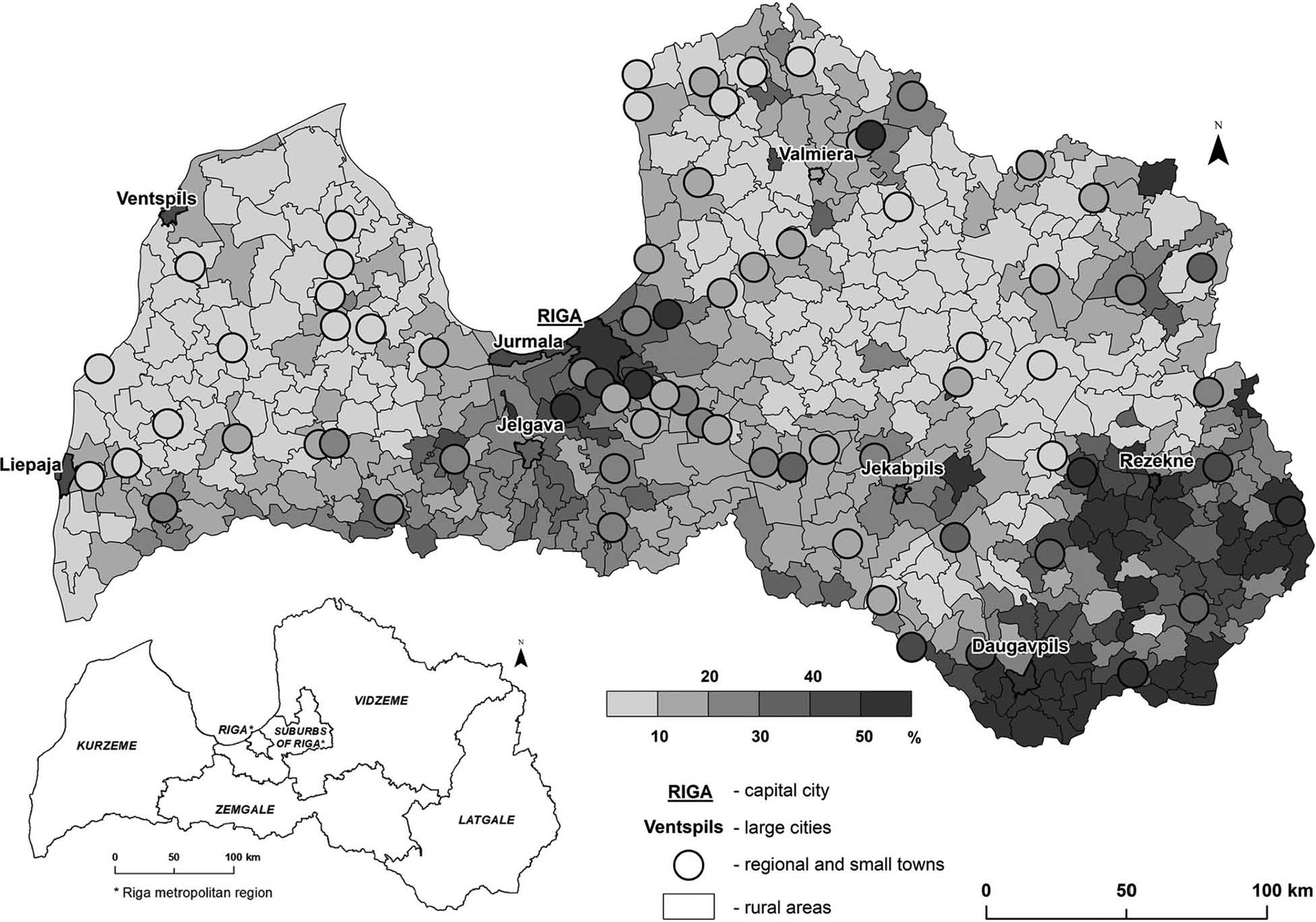
Fig. 1.
The share (%) of ethnic minorities by territorial units (urban and rural) in Latvia (2019) based on data from the Central Statistical Bureau of Latvia.
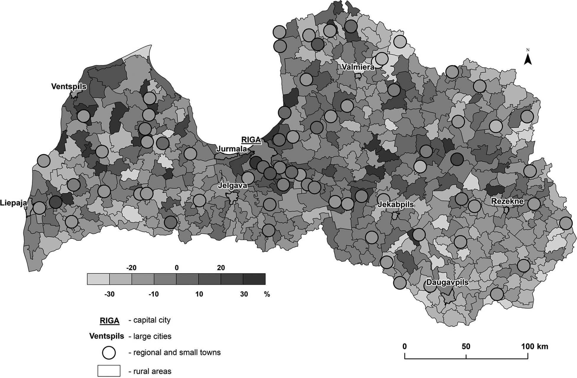
Fig. 2.
Relative population change (100% = 2011) among ethnic minorities by territorial units (urban and rural) in Latvia (2011–2019) based on data from the Central Statistical Bureau of Latvia.
Table 2.
In-migrants and non-migrants by ethnicity (age group 0–14 excluded).
| 2010–2011 | 2018–2019 | |||||||
|---|---|---|---|---|---|---|---|---|
| In-migrants | Non-migrants | In-migrants | Non-migrants | |||||
| Count (k) | % | Count (k) | % | Count (k) | % | Count (k) | % | |
| Latvians | 33.6 | 3.3 | 999.9 | 96.7 | 32.8 | 3.4 | 943.7 | 96.6 |
| Ethnic minorities | 14.0 | 2.0 | 668.4 | 98.0 | 12.2 | 2.0 | 600.7 | 98.0 |
| Total | 47.6 | 2.8 | 1668.3 | 97.2 | 45.0 | 2.8 | 1544.4 | 97.2 |
Table 3.
Binary logistic regression model variables.
| Type | Variable | Group | Regression model no. |
|---|---|---|---|
| Filter variables | Ethnicity | Latvians | all |
| Ethnic minorities | |||
| Dependent variable | Migration status | In-migrants | all |
| Non-migrants | |||
| Covariates (predictor variables) | Age group | 15–19 | all |
| 20–24 | |||
| 25–29 | |||
| 30–34 | |||
| 35–39 | |||
| 40+ | |||
| Urban system | Capital city of Riga | 1; 2; 3; 4 | |
| Suburbs of Riga | |||
| Other largest cities | |||
| Regional & small towns | |||
| Rural areas | |||
| Region | Riga & suburbs | 5; 6; 7; 8 | |
| Zemgale | |||
| Vidzeme Kurzeme | |||
| Latgale |
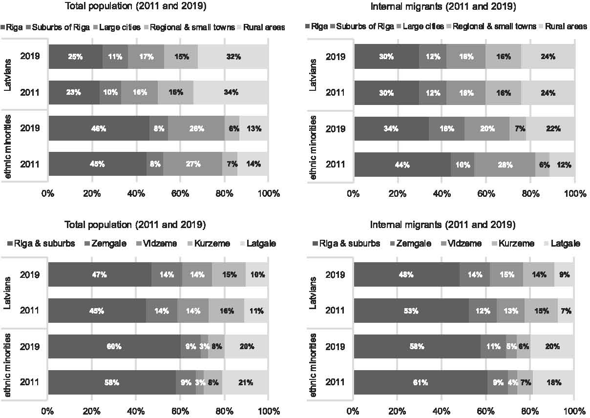
Fig. 3.
Distribution of the total population and internal migrants across the urban system and regions by the majority-minority ethnic groups (2011 and 2019) based on data from the Population Census (2011) and Population Register (2019).
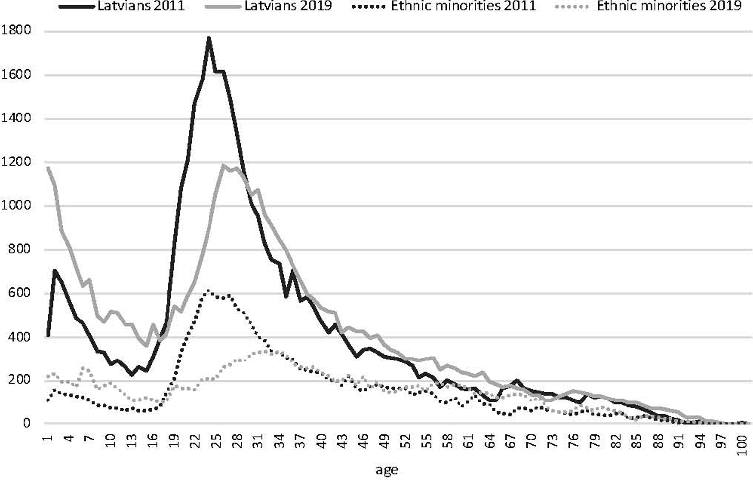
Fig. 4.
Age-specific migration propensities by majority-minority ethnic groups (2011 and 2019) based on data from the Population Census (2011) and Population Register (2019).
Table 4.
Logistic regression of the likelihood of internal migration, predicted by age group and destination within the urban system (ref. non-migrants Latvians).
| β – internal migrants among Latvians (ref. non-migrants) | |||||
|---|---|---|---|---|---|
| Model 1 (2011) | Model 2 (2019) | ||||
| β coefficient | P | β coefficient | P | ||
| Age | 15–19 | −0.139 | 0.000 | 0.194 | 0.000 |
| 20–24 | 0.914 | 0.000 | 0.754 | 0.000 | |
| 25–29 | 1.000 | (ref.) | 1.000 | (ref.) | |
| 30–34 | 0.543 | 0.000 | 0.845 | 0.000 | |
| 35–39 | 0.102 | 0.000 | 0.531 | 0.000 | |
| 40+ | −0.620 | 0.000 | −0.254 | 0.000 | |
| Urban system | Capital city of Riga | 1.000 | (ref.) | 1.000 | (ref.) |
| Suburbs of Riga | 0.872 | 0.000 | 1.178 | 0.000 | |
| Large cities | 0.807 | 0.000 | 0.940 | 0.007 | |
| Regional & small towns | 0.758 | 0.000 | 1.064 | 0.025 | |
| Rural areas | 0.471 | 0.000 | 0.976 | 0.127 | |
| −2 Log likelihood | 279,745.547 | 276,813.279 | |||
| Nagelkerke R2 | 0.065 | 0.041 | |||
1 Note: Values reported are β coefficients on the log-odds scale. Corresponding odds ratios are obtained as OR = exp(β); e.g., β = 0.914 corresponds to OR ≈ 2.49, and β = −0.620 to OR ≈ 0.54. Because the data approximate the full resident population, p-values are reported for completeness and should be read as descriptive markers of effect magnitude rather than as inferential tests against sampling error (Mood 2010).
Table 5.
Logistic regression of the likelihood of internal migration, predicted by age group and destination within the urban system (ref. non-migrants ethnic minorities).
| β – internal migrants among ethnic minorities (ref. non-migrants) | |||||
|---|---|---|---|---|---|
| Model 3 (2011) | Model 4 (2019) | ||||
| β coefficient | P | β coefficient | P | ||
| Age | 15–19 | −0.183 | 0.000 | 0.180 | 0.000 |
| 20–24 | 0.904 | 0.001 | 0.816 | 0.000 | |
| 25–29 | 1.000 | (ref.) | 1.000 | (ref.) | |
| 30–34 | 0.636 | 0.000 | 0.913 | 0.020 | |
| 35–39 | 0.194 | 0.000 | 0.680 | 0.000 | |
| 40+ | −0.693 | 0.000 | −0.123 | 0.000 | |
| Urban system | Capital city of Riga | 1.000 | (ref.) | 1.000 | (ref.) |
| Suburbs of Riga | 1.090 | 0.000 | 1.428 | 0.000 | |
| Large cities | 0.953 | 0.286 | 1.414 | 0.000 | |
| Regional & small towns | 0.956 | 0.512 | 1.851 | 0.000 | |
| Rural areas | 0.928 | 0.011 | 1.828 | 0.000 | |
| −2 Log likelihood | 129,068.467 | 114,064.836 | |||
| Nagelkerke R2 | 0.059 | 0.052 | |||
1 Note: Values reported are β coefficients on the log-odds scale. Corresponding odds ratios are obtained as OR = exp(β); e.g., β = 0.914 corresponds to OR ≈ 2.49, and β = −0.620 to OR ≈ 0.54. Because the data approximate the full resident population, p-values are reported for completeness and should be read as descriptive markers of effect magnitude rather than as inferential tests against sampling error (Mood 2010).
Table 6.
Logistic regression of the likelihood of internal migration, predicted by age group and region of destination (ref. non-migrants Latvians).
| β – internal migrants among Latvians (ref. non-migrants) | |||||
|---|---|---|---|---|---|
| Model 5 (2011) | Model 6 (2019) | ||||
| β coefficient | P | β coefficient | P | ||
| Age | 15–19 | −0.167 | 0.000 | 0.220 | 0.000 |
| 20–24 | 0.895 | 0.000 | 0.762 | 0.000 | |
| 25–29 | 1.000 | (ref.) | 1.000 | (ref.) | |
| 30–34 | 0.544 | 0.000 | 0.853 | 0.000 | |
| 35–39 | 0.096 | 0.000 | 0.556 | 0.000 | |
| 40+ | −0.638 | 0.000 | −0.243 | 0.000 | |
| Regions | Riga & suburbs | 1.000 | (ref.) | 1.000 | (ref.) |
| Zemgale | 0.739 | 0.000 | 0.869 | 0.000 | |
| Kurzeme | 0.807 | 0.000 | 0.930 | 0.000 | |
| Vidzeme | 0.782 | 0.000 | 0.777 | 0.000 | |
| Latgale | 0.515 | 0.000 | 0.624 | 0.000 | |
| −2 Log likelihood | 280,393.782 | 277,992.085 | |||
| Nagelkerke R2 | 0.062 | 0.037 | |||
1 Note: Values reported are β coefficients on the log-odds scale. Corresponding odds ratios are obtained as OR = exp(β); e.g., β = 0.895 corresponds to OR ≈ 2.45, and β = −0.638 to OR ≈ 0.53. Because the data approximate the full resident population, p-values are reported for completeness and should be read as descriptive markers of effect magnitude rather than as inferential tests against sampling error (Mood 2010).
Table 7.
Logistic regression of the likelihood of internal migration, predicted by age group and region of destination (ref. non-migrants ethnic minorities).
| β – internal migrants among minorities (ref. non-migrants) | |||||
|---|---|---|---|---|---|
| Model 7 (2011) | Model 8 (2019) | ||||
| β coefficient | P | β coefficient | P | ||
| Age | 15–19 | −0.174 | 0.000 | 0.227 | 0.000 |
| 20–24 | 0.906 | 0.001 | 0.851 | 0.001 | |
| 25–29 | 1.000 | (ref.) | 1.000 | (ref.) | |
| 30–34 | 0.639 | 0.000 | 0.908 | 0.013 | |
| 35–39 | 0.201 | 0.000 | 0.704 | 0.000 | |
| 40+ | −0.698 | 0.000 | −0.088 | 0.000 | |
| Regions | Riga & suburbs | 1.000 | (ref.) | 1.000 | (ref.) |
| Zemgale | 0.975 | 0.402 | 1.222 | 0.000 | |
| Kurzeme | 1.275 | 0.000 | 1.254 | 0.000 | |
| Vidzeme | 0.858 | 0.000 | 0.695 | 0.000 | |
| Latgale | 0.861 | 0.000 | 0.852 | 0.000 | |
| −2 Log likelihood | 129,127.080 | 117,087.907 | |||
| Nagelkerke R2 | 0.058 | 0.025 | |||
1 Note: Values reported are β coefficients on the log-odds scale. Corresponding odds ratios are obtained as OR = exp(β); e.g., β = 0.914 corresponds to OR ≈ 2.49, and β = −0.620 to OR ≈ 0.54. Because the data approximate the full resident population, p-values are reported for completeness and should be read as descriptive markers of effect magnitude rather than as inferential tests against sampling error (Mood 2010).