
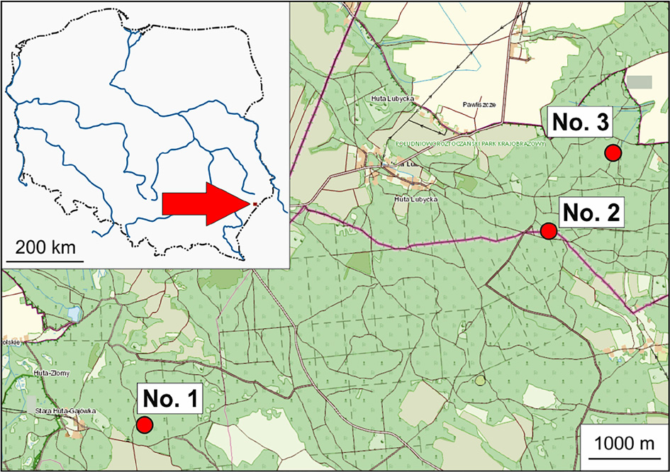
Fig. 1.
Location of the study area (background map source: WMS and WMTS viewing services, Central Office of Geodesy and Cartography, Poland).
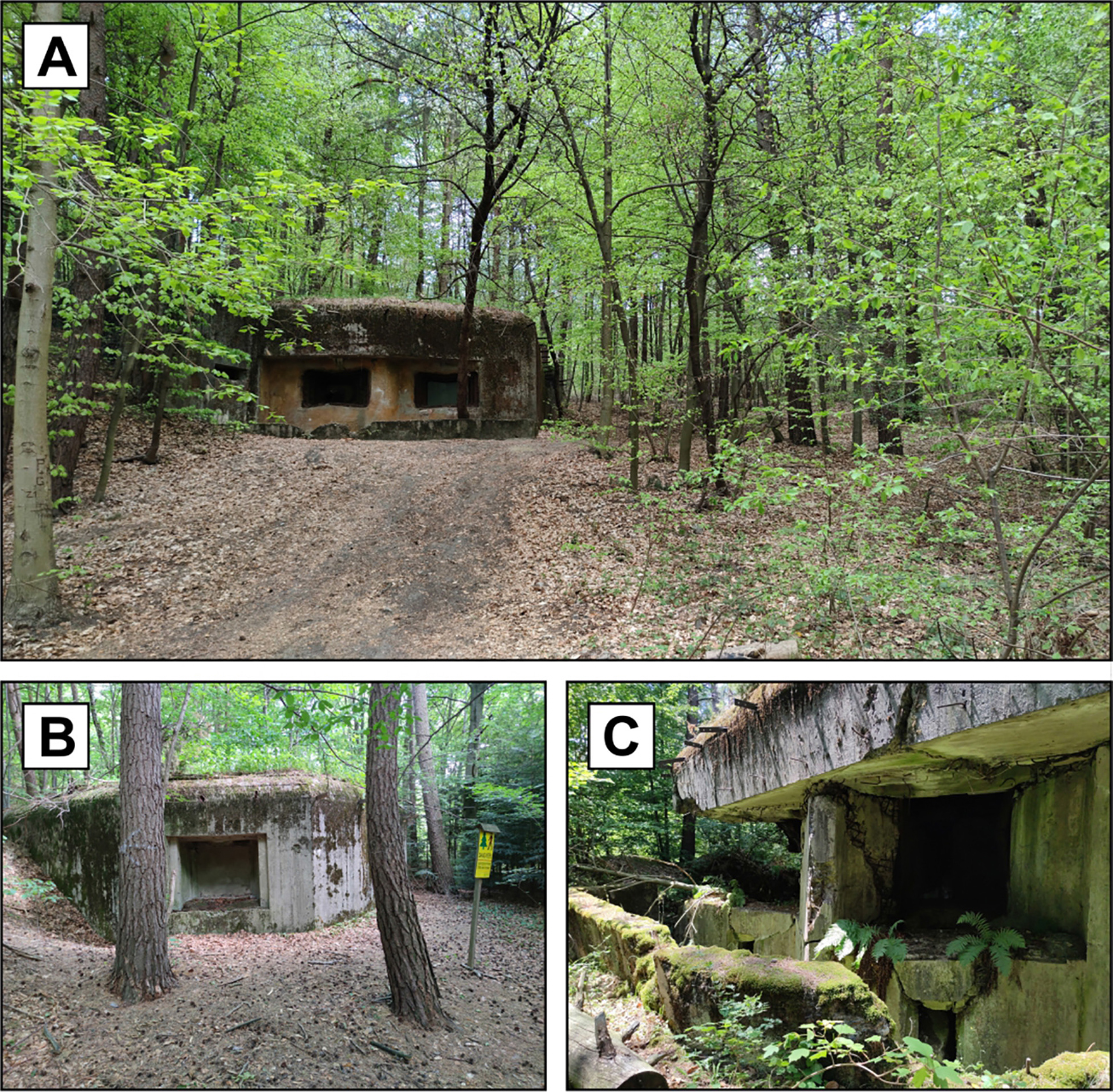
Fig. 2.
Selected bunkers of the Rava-Russkaia Fortified Region of the Molotov Line. A – Bunker No. 1 – tourists visiting a bunker on the Molotov Line, B – Front wall of unfinished bunker No. 2, C – Bunker No. 3 damaged by shelling and experimental explosion (photo by G. Gajek).
Table 1.
Basic physicochemical properties of studied soils.
| Parameter | Unit | Mean | Median | Min | Max | SD |
|---|---|---|---|---|---|---|
| Bunker No. 1 | ||||||
| pH (H2O) | – | 4.7 | 4.2 | 3.5 | 7.5 | 1.3 |
| Sand (grain diameters 2–0.05 mm) | % | 93.1 | 93.2 | 89.0 | 97.1 | 2.2 |
| Silt (grain diameters 0.05–0.002 mm) | 6.8 | 6.7 | 3.0 | 10.0 | 2.0 | |
| Clay (grain diameters <0.002 mm) | 0.1 | 0.0 | 0.0 | 0.8 | 0.2 | |
| Total organic carbon TOC | g · kg-1 | 13.0 | 12.0 | 5.0 | 34.0 | 0.8 |
| Hydrolytic acidity HA | cmol(+) · kg-1 | 4.4 | 4.1 | 0.8 | 11.2 | 2.4 |
| Base exchange capacity BEC | 5.1 | 4.0 | 2.0 | 16.7 | 3.7 | |
| Effective cation exchange capacity ECEC | 9.5 | 9.1 | 5.1 | 20.2 | 4.1 | |
| 0–20 cm | ||||||
| Bi | mg · kg-1 | 4.9 | 4.8 | 0.0 | 4.9 | – |
| Cd | 0.3 | 0.2 | 0.1 | 1.0 | 0.2 | |
| Cr | 11.1 | 8.9 | 0.0 | 30.6 | 9.5 | |
| Cu | 4.3 | 3.6 | 0.6 | 16.0 | 3.5 | |
| Mn | 94.7 | 72.7 | 15.1 | 337.6 | 79.3 | |
| Ni | 7.0 | 5.4 | 0.0 | 21.5 | 6.5 | |
| Pb | 16.2 | 9.7 | 1.8 | 143.0 | 29.3 | |
| Zn | 26.4 | 20.2 | 8.5 | 98.4 | 20.2 | |
| 20–40 cm | ||||||
| Bi | mg · kg-1 | – | – | – | – | – |
| Cd | 0.3 | 0.2 | 0.1 | 1.4 | 0.3 | |
| Cr | 11.0 | 8.5 | 0.3 | 38.5 | 11.5 | |
| Cu | 3.4 | 2.0 | 0.6 | 6.3 | 4.5 | |
| Mn | 163.1 | 182.4 | 14.4 | 320.1 | 95.5 | |
| Ni | 10.6 | 6.5 | 1.2 | 38.5 | 12.1 | |
| Pb | 4.2 | 4.3 | 1.2 | 8.9 | 2.1 | |
| Zn | 15.2 | 11.6 | 3.7 | 37.1 | 9.1 | |
| Bunker No. 2 | ||||||
| pH (H2O) | – | 4.3 | 3.9 | 3.5 | 7.2 | 1.0 |
| Sand (grain diameters 2–0.05 mm) | % | 94.7 | 94.2 | 88.0 | 99.9 | 3.7 |
| Silt (grain diameters 0.05–0.002 mm) | 4.9 | 5.6 | 0.0 | 11.6 | 3.8 | |
| Clay (grain diameters <0.002 mm) | 0.1 | 0.1 | 0.0 | 0.5 | 0.2 | |
| Total organic carbon TOC | g · kg-1 | 16.0 | 16.0 | 3.0 | 49.0 | 1.2 |
| Hydrolytic acidity HA | cmol(+) · kg-1 | 4.1 | 3.6 | 0.9 | 11.7 | 2.4 |
| Base exchange capacity BEC | 2.7 | 1.8 | 0.5 | 9.9 | 2.4 | |
| Effective cation exchange capacity ECEC | 6.4 | 5.9 | 2.3 | 13.8 | 3.3 | |
| 0–20 cm | ||||||
| Bi | mg · kg-1 | 5.3 | 4.6 | 1.8 | 20.0 | 5.0 |
| Cd | 0.3 | 0.2 | 0.1 | 1.0 | 0.2 | |
| Cr | 33.0 | 33.6 | 18.5 | 44.2 | 7.9 | |
| Cu | 3.3 | 2.3 | 1.1 | 9.8 | 2.3 | |
| Mn | 102.3 | 36.6 | 12.1 | 533.9 | 137.1 | |
| Ni | 15.9 | 16.1 | 10.3 | 23.4 | 3.2 | |
| Pb | 13.3 | 12.2 | 4.2 | 35.8 | 6.8 | |
| Zn | 25.5 | 20.8 | 13.0 | 70.1 | 13.0 | |
| 20–40 cm | ||||||
| Bi | mg · kg-1 | 4.5 | 3.8 | 0.0 | 8.2 | 2.1 |
| Cd | 0.2 | 0.1 | 0.0 | 0.5 | 0.1 | |
| Cr | 32.1 | 34.5 | 18.9 | 42.9 | 7.7 | |
| Cu | 1.8 | 1.3 | 0.0 | 7.2 | 1.6 | |
| Mn | 97.6 | 72.5 | 7.8 | 447.2 | 104.1 | |
| Ni | 14.8 | 14.7 | 10.4 | 22.9 | 3.0 | |
| Pb | 3.9 | 3.1 | 1.3 | 11.1 | 2.6 | |
| Zn | 12.8 | 10.6 | 3.5 | 30.3 | 7.4 | |
| Bunker No. 3 | ||||||
| pH (H2O) | – | 4.3 | 3.9 | 3.6 | 7.8 | 1.1 |
| Sand (grain diameters 2–0.05 mm) | % | 80.1 | 79.8 | 71.4 | 90.0 | 5.7 |
| Silt (grain diameters 0.05–0.002 mm) | 18.8 | 19.1 | 9.4 | 27.2 | 5.5 | |
| Clay (grain diameters <0.002 mm) | 1.1 | 1.2 | 0.3 | 1.4 | 0.3 | |
| Total organic carbon TOC | g · kg-1 | 9.0 | 6.0 | 2.0 | 28.0 | 1.8 |
| Hydrolytic acidity HA | cmol(+) · kg-1 | 4.2 | 3.4 | 1.5 | 9.6 | 2.2 |
| Base exchange capacity BEC | 3.9 | 1.1 | 0.3 | 29.0 | 7.4 | |
| Effective cation exchange capacity ECEC | 8.1 | 4.7 | 2.7 | 38.6 | 8.7 | |
| 0-20 cm | ||||||
| Bi | mg · kg-1 | 6.2 | 5.2 | 0.0 | 11.7 | 3.8 |
| Cd | 0.2 | 0.1 | 0.0 | 1.3 | 0.3 | |
| Cr | 15.1 | 14.1 | 11.8 | 34.5 | 4.9 | |
| Cu | 1.4 | 0.9 | 0.0 | 9.0 | 2.1 | |
| Mn | 26.4 | 11.7 | 6.1 | 130.1 | 33.9 | |
| Ni | 9.4 | 8.7 | 7.2 | 19.0 | 2.6 | |
| Pb | 5.2 | 4.3 | 0.6 | 10.6 | 2.6 | |
| Zn | 12.0 | 11.5 | 2.9 | 44.1 | 9.1 | |
| 20-40 cm | ||||||
| Bi | mg · kg-1 | 0.6 | 0.2 | 0.0 | 10.0 | 2.2 |
| Cd | 0.2 | 0.1 | 0.0 | 1.0 | 0.2 | |
| Cr | 15.3 | 15.2 | 11.2 | 23.7 | 2.7 | |
| Cu | 0.6 | 0.2 | 0.0 | 5.5 | 1.3 | |
| Mn | 59.3 | 38.6 | 6.0 | 186.4 | 54.6 | |
| Ni | 9.3 | 9.4 | 7.3 | 15.7 | 1.9 | |
| Pb | 2.7 | 2.3 | 0.7 | 8.3 | 1.6 | |
| Zn | 8.2 | 7.0 | 1.7 | 29.9 | 5.9 | |
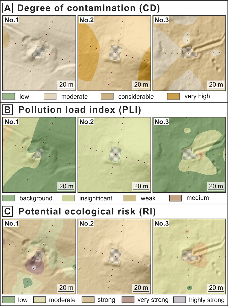
Fig. 3.
Pollution index PI values calculated from the content of selected trace metals TMs in the 0–20 cm horizon; A – Degree of contamination (CD); B – Pollution load index (PLI); C – Potential ecological risk (RI) (background map source: WMS and WMTS viewing services, Central Office of Geodesy and Cartography, Poland).
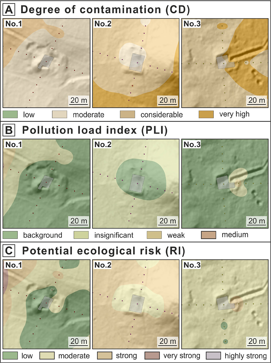
Fig. 4.
Pollution index PI values calculated from the content of selected trace metals TMs in the 20-40 cm horizon; A – Degree of contamination (CD); B – Pollution load index (PLI); C – Potential ecological risk (RI) (background map source: WMS and WMTS viewing services, Central Office of Geodesy and Cartography, Poland).
Table 2.
Igeo of bunker No. 2.
| Depth Sample number* | Zn | Mn | Cu | Ni | Cd | Cr | Pb | |||||||
|---|---|---|---|---|---|---|---|---|---|---|---|---|---|---|
| 0–20 | 20–40 | 0–20 | 20–40 | 0–20 | 20–40 | 0–20 | 20–40 | 0–20 | 20–40 | 0–20 | 20–40 | 0–20 | 20–40 | |
| [cm] | ||||||||||||||
| 2\0\0 | 1.09 | –1.79 | 1.64 | –1.89 | 0.38 | –3.70 | 1.96 | 1.43 | 0.43 | –2.91 | 2.80 | 2.50 | 1.41 | –2.17 |
| 2\N\10 | –0.74 | –2.20 | –2.95 | –4.06 | –2.15 | –4.64 | 1.48 | 1.07 | –2.12 | –3.68 | 2.83 | 2.05 | –0.35 | –2.55 |
| 2\N\20 | –1.32 | –1.88 | –3.82 | –2.03 | –2.02 | –4.64 | 1.20 | 1.22 | –2.47 | –2.44 | 2.27 | 2.56 | –1.46 | –1.19 |
| 2\N\30 | –0.67 | –0.23 | –1.91 | 1.39 | –1.61 | –1.56 | 0.78 | 1.03 | –2.51 | –1.56 | 1.63 | 1.83 | –0.75 | –0.45 |
| 2\N\40 | –0.69 | –0.82 | –2.15 | –0.34 | –2.19 | –2.76 | 0.94 | 0.93 | –2.64 | –2.44 | 1.66 | 1.74 | –0.09 | –2.06 |
| 2\N\50 | –0.45 | –0.92 | –1.98 | –1.10 | –1.69 | –2.41 | 0.98 | 0.79 | –1.99 | –3.18 | 1.75 | 1.66 | 0.05 | –2.38 |
| 2\W\10 | –0.29 | –1.84 | –2.43 | –2.10 | –1.03 | –3.22 | 0.85 | 0.84 | –0.81 | –2.03 | 2.20 | 1.67 | –0.34 | –3.14 |
| 2\W\20 | –0.03 | –1.66 | 1.23 | –0.14 | –2.74 | –2.47 | 1.36 | 1.12 | –1.54 | –2.90 | 2.44 | 2.32 | 0.47 | –2.48 |
| 2\W\30 | –0.78 | –1.60 | –3.09 | –0.71 | –0.98 | –2.33 | 1.40 | 1.15 | –2.90 | –3.91 | 2.50 | 2.63 | –0.04 | –1.07 |
| 2\W\40 | 0.44 | –1.66 | –2.57 | 0.79 | –0.08 | –2.55 | 1.36 | 1.44 | –3.22 | –2.35 | 2.62 | 2.76 | –0.25 | –2.34 |
| 2\W\50 | –1.03 | –1.17 | 0.60 | –1.39 | –2.79 | –1.95 | 1.66 | 1.52 | –1.92 | –3.91 | 2.72 | 2.58 | –1.67 | –0.29 |
| 2\S\10 | 0.07 | –1.46 | –3.73 | –1.82 | –2.17 | –3.27 | 1.40 | 1.50 | –2.21 | –3.17 | 2.84 | 2.80 | –0.93 | –2.29 |
| 2\S\20 | 0.20 | –0.12 | –2.30 | –0.63 | –0.53 | –1.00 | 1.49 | 1.50 | –2.08 | –2.92 | 2.59 | 2.60 | –0.16 | –1.37 |
| 2\S\30 | –1.06 | –1.19 | –1.04 | –0.51 | –2.00 | –3.13 | 1.46 | 1.48 | –3.73 | –2.44 | 2.45 | 2.84 | 0.09 | –3.40 |
| 2\S\40 | –0.83 | –1.43 | –0.02 | –0.44 | –1.81 | –3.26 | 1.52 | 1.48 | –1.95 | –2.92 | 2.56 | 2.55 | –0.51 | –2.02 |
| 2\S\50 | –0.82 | –0.46 | –0.36 | –0.06 | –1.72 | –1.74 | 1.61 | 1.62 | –2.45 | –1.44 | 2.61 | 2.60 | –0.13 | –2.07 |
| 2\E\10 | –0.66 | –3.24 | –3.60 | –4.19 | –2.33 | –3.93 | 1.46 | 1.33 | –2.33 | –3.91 | 2.45 | 2.47 | –0.14 | –3.35 |
| 2\E\20 | –1.26 | –2.89 | –2.92 | –4.46 | –2.21 | –4.64 | 1.42 | 1.24 | –3.13 | –3.64 | 2.35 | 2.30 | –0.44 | –1.77 |
| 2\E\30 | –1.35 | –1.82 | –3.39 | –3.88 | –1.43 | –4.64 | 1.43 | 1.27 | –1.39 | –2.80 | 2.75 | 2.59 | 0.66 | –2.09 |
| 2\E\40 | –0.47 | –3.06 | –3.14 | –3.63 | –1.28 | –2.01 | 1.49 | 1.32 | –1.45 | –2.40 | 2.47 | 2.48 | 0.60 | –2.31 |
| 2\E\50 | –0.47 | –0.92 | –0.35 | –1.03 | –0.31 | –0.06 | 1.85 | 1.93 | –0.05 | –0.48 | 2.88 | 2.77 | 0.47 | –1.12 |
| Unpolluted | Unpolluted to moderately polluted | Moderately polluted | Moderately to strongly polluted | |||||||||||
Table 3.
Igeo of bunker No. 1.
| Depth Sample number* | Zn | Mn | Cu | Ni | Cd | Cr | Pb | |||||||
|---|---|---|---|---|---|---|---|---|---|---|---|---|---|---|
| 0–20 | 20–40 | 0–20 | 20–40 | 0–20 | 20–40 | 0–20 | 20–40 | 0–20 | 20–40 | 0–20 | 20–40 | 0–20 | 20–40 | |
| [cm] | ||||||||||||||
| 1\0\0 | 1.58 | –0.55 | –0.02 | –2.16 | 0.02 | –3.69 | –2.90 | –2.91 | –0.07 | –2.20 | –4.32 | –4.32 | 0.62 | –1.33 |
| 1\N\10 | –0.78 | –1.42 | –2.61 | 0.09 | –1.26 | –1.40 | –2.91 | –2.91 | –1.79 | –1.17 | –4.32 | –4.28 | –0.44 | –1.67 |
| 1\N\20 | –0.88 | –1.08 | –.32 | 0.82 | –1.07 | –0.76 | –2.91 | –2.36 | –1.78 | –1.71 | –4.32 | –4.32 | –0.39 | –0.82 |
| 1\N\30 | –1.28 | –0.15 | –0.73 | 0.90 | –1.50 | 0.23 | –2.91 | 1.46 | –1.87 | 0.23 | –4.32 | 0.57 | –0.88 | –1.09 |
| 1\N\40 | –1.21 | –1.51 | –1.76 | 0.23 | –1.52 | –1.83 | –2.91 | –2.91 | –1.99 | –1.18 | –4.32 | –4.32 | –0.48 | –2.57 |
| 1\N\50 | –1.53 | –1.96 | –1.49 | 0.19 | –1.93 | –3.51 | –0.43 | –0.35 | –2.06 | –1.93 | 0.12 | 0.09 | –0.35 | –2.91 |
| 1\W\10 | –0.66 | –3.16 | –3.22 | –2.43 | –1.77 | –2.39 | –0.53 | –0.40 | –1.69 | –2.45 | 0.35 | 0.21 | –0.33 | –3.47 |
| 1\W\20 | 0.00 | –2.04 | –1.41 | –2.40 | –0.58 | –1.89 | 0.33 | 0.16 | –0.78 | –1.56 | 0.72 | 0.51 | –0.49 | –2.56 |
| 1\W\30 | 0.10 | –1.71 | –0.64 | –0.25 | 0.13 | –1.15 | 0.70 | 0.14 | –0.44 | –1.18 | 1.24 | 0.74 | –0.04 | –1.61 |
| 1\W\40 | –0.94 | –1.25 | –1.94 | 0.56 | –0.96 | –1.27 | 0.01 | 0.11 | –1.34 | –1.07 | 0.58 | 0.50 | –0.39 | –1.24 |
| 1\W\50 | 0.74 | 0.17 | 0.98 | 0.71 | 1.09 | 1.50 | 1.84 | 2.68 | 0.45 | 0.85 | 2.35 | 2.68 | 0.21 | –0.60 |
| 1\S\10 | 0.18 | –1.67 | –0.40 | 0.51 | 0.01 | –2.29 | –2.91 | –2.91 | –1.18 | –2.70 | –4.20 | –4.32 | 3.41 | –1.52 |
| 1\S\20 | –0.70 | –1.01 | –0.42 | 0.47 | –1.21 | –1.80 | –2.91 | –2.91 | –2.21 | –2.40 | –4.32 | –4.32 | 0.26 | –1.35 |
| 1\S\30 | –1.78 | –1.49 | –2.28 | –0.13 | –2.39 | –2.50 | –2.91 | –2.91 | –3.08 | –2.72 | –4.32 | –4.32 | –1.10 | –2.01 |
| 1\S\40 | –1.15 | –1.94 | –2.39 | –0.72 | –2.10 | –2.31 | –2.91 | –2.91 | –2.95 | –3.30 | –4.32 | –4.32 | –0.80 | –2.14 |
| 1\S\50 | –1.38 | –0.34 | –0.94 | –0.76 | –2.54 | –1.32 | –2.91 | –2.91 | –2.84 | –2.93 | –4.32 | –4.32 | –0.68 | –2.76 |
| 1\E\10 | –0.21 | 0.00 | –2.40 | 0.35 | –0.87 | –0.56 | –2.91 | –2.91 | –2.25 | –1.63 | –4.32 | –4.32 | –0.93 | –1.03 |
| 1\E\20 | –0.50 | –1.64 | –1.23 | –2.46 | –0.81 | –2.48 | –2.91 | –2.91 | –2.21 | –2.80 | –4.32 | –4.32 | –0.43 | –4.75 |
| 1\E\30 | 0.30 | –1.68 | 0.08 | –0.30 | –0.08 | –2.44 | –1.83 | –2.91 | –1.44 | –1.92 | –4.32 | –4.32 | –0.80 | –1.55 |
| 1\E\40 | –0.40 | –1.61 | –3.27 | 0.24 | –0.93 | –2.33 | –2.91 | –2.91 | –2.79 | –3.46 | –4.32 | –4.32 | –0.66 | –3.01 |
| 1\E\50 | –1.85 | –1.96 | –3.51 | –3.57 | –3.08 | –2.23 | –2.91 | –2.91 | –2.93 | –3.91 | –4.32 | –4.32 | –1.31 | –2.23 |
| Unpolluted | Unpolluted to moderately polluted | Moderately polluted | Moderately to strongly polluted | Highly polluted | ||||||||||
Table 4.
Igeo of bunker No. 3.
| Depth Sample number* | Zn | Mn | Cu | Ni | cd | Cr | Pb | |||||||
|---|---|---|---|---|---|---|---|---|---|---|---|---|---|---|
| 0-20 | 20–40 | 0–20 | 20–40 | 0–20 | 20–40 | 0–20 | 20–40 | 0–20 | 20–40 | 0–20 | 20–40 | 0–20 | 20–40 | |
| [cm] | ||||||||||||||
| 3\0\0 | –0.24 | –2.65 | –1.24 | –0.78 | –2.15 | –4.64 | 1.08 | 0.84 | –1.38 | –2.53 | 1.82 | 1.54 | –0.29 | –1.96 |
| 3\N\10 | –1.14 | –2.01 | –2.93 | –0.94 | –1.82 | –4.64 | 0.99 | 0.96 | –2.35 | –2.80 | 1.57 | 1.58 | –1.86 | –3.00 |
| 3\N\20 | –0.94 | –1.50 | –3.77 | –0.31 | –0.69 | –1.63 | 0.78 | 0.71 | –2.19 | –3.14 | 1.34 | 1.31 | –0.34 | –2.75 |
| 3\N\30 | –3.15 | –3.33 | –4.49 | –1.63 | –4.64 | –4.64 | 0.39 | 0.42 | –3.00 | –2.96 | 1.03 | 1.06 | –2.07 | –2.31 |
| 3\N\40 | –2.25 | –3.28 | –4.13 | –2.51 | –4.64 | –4.64 | 0.41 | 0.62 | –2.84 | –3.82 | 1.08 | 1.22 | –1.73 | –2.65 |
| 3\N\50 | –3.13 | –2.49 | –3.62 | –4.40 | –3.17 | –4.39 | 0.61 | 0.68 | –3.10 | –2.90 | 1.31 | 1.22 | –1.86 | –2.42 |
| 3\W\10 | –2.40 | –2.83 | –4.09 | –2.17 | –2.99 | –4.64 | 0.76 | 0.70 | –2.37 | –1.17 | 1.21 | 1.25 | –1.44 | –2.31 |
| 3\W\20 | –1.44 | –2.94 | –4.13 | –3.88 | –3.03 | –2.75 | 0.46 | 0.40 | –1.11 | –0.75 | 1.30 | 1.47 | –1.58 | –2.79 |
| 3\W\30 | –1.24 | –2.53 | –4.36 | –3.93 | –2.44 | –4.64 | 0.46 | 0.28 | –2.28 | –1.94 | 1.16 | 1.08 | –0.64 | –3.14 |
| 3\W\40 | –2.00 | –2.00 | –4.82 | –4.31 | –4.64 | –4.64 | 0.27 | 0.35 | –1.76 | –0.69 | 1.06 | 1.37 | –1.94 | –2.25 |
| 3\W\50 | –0.98 | –2.40 | –4.47 | –4.14 | –4.64 | –4.64 | 0.26 | 0.54 | –1.55 | –1.12 | 1.33 | 1.55 | –1.98 | –2.21 |
| 3\S\10 | –0.81 | –2.19 | –0.39 | –1.25 | –1.44 | –4.64 | 0.68 | 0.43 | –0.72 | –2.17 | 1.06 | 1.02 | –0.73 | –2.67 |
| 3\S\20 | –1.45 | –3.82 | –4.23 | –2.13 | –2.12 | –4.64 | 0.47 | 0.28 | –2.83 | –3.19 | 1.11 | 1.02 | –2.20 | –3.45 |
| 3\S\30 | –3.16 | –1.80 | –3.96 | –1.07 | –4.64 | –4.64 | 0.31 | 0.33 | –3.91 | –1.17 | 1.05 | 1.37 | –1.88 | –3.05 |
| 3\S\40 | –3.51 | –4.28 | –2.16 | –4.82 | –3.81 | –4.64 | 0.42 | 0.41 | –2.93 | –3.91 | 1.08 | 1.24 | –4.52 | –4.25 |
| 3\S\50 | –2.40 | –2.27 | –4.22 | –2.64 | –4.64 | –4.64 | 0.45 | 0.37 | –2.92 | –2.49 | 0.98 | 0.90 | –1.42 | –1.15 |
| 3\E\10 | 0.42 | –0.14 | –0.64 | –0.35 | 0.27 | –0.45 | 1.66 | 1.39 | 0.82 | 0.39 | 2.52 | 1.98 | –0.43 | –0.71 |
| 3\E\20 | –1.51 | –1.56 | –3.28 | –0.88 | –4.64 | –4.64 | 0.76 | 0.71 | –2.60 | –3.91 | 1.42 | 1.41 | –0.64 | –2.20 |
| 3\E\30 | –2.00 | –2.00 | –3.57 | 0.12 | –4.64 | –3.19 | 0.65 | 0.68 | –3.91 | –2.59 | 1.26 | 1.35 | –1.51 | –2.95 |
| 3\E\40 | –1.52 | –1.54 | –2.11 | –4.61 | –2.68 | –2.78 | 0.67 | 0.67 | –3.91 | –3.78 | 1.29 | 1.34 | –1.94 | –2.41 |
| 3\E\50 | –1.02 | –1.84 | –2.07 | –0.12 | –1.88 | –2.31 | 0.90 | 0.86 | –2.97 | –2.85 | 1.54 | 1.47 | –1.30 | –1.88 |
| Unpolluted | Unpolluted to moderately polluted | Moderately polluted | Moderately to strongly polluted | |||||||||||
Table 5.
PCA results for bunkers. Principal components as groups of similar origin. Numbers in columns are influence of each data on the given principal component.
| Parameter | Group 1 (first principal component) | Group 2 (second principal component) | Group 3 (third principal component) | Group 4 (fourth principal component) |
|---|---|---|---|---|
| Cu | -0.85611 | 0.306189 | 0.096109 | -0.242390 |
| Ni | -0.54351 | -0.822840 | -0.103110 | -0.023880 |
| Cd | -0.85712 | 0.127119 | 0.246373 | -0.129310 |
| Cr | -0.48870 | -0.841140 | -0.179290 | -0.055030 |
| Pb | -0.38842 | 0.415467 | -0.818640 | 0.007732 |
| Zn | -0.82996 | 0.298641 | 0.110614 | -0.154310 |
| Mn | -0.74662 | 0.104419 | 0.102310 | 0.647287 |
| Partial variation [%] | 48.6 | 25.2 | 11.5 | 7.5 |
| Summarised variation [%] | 48.6 | 73.8 | 85.3 | 92.8 |
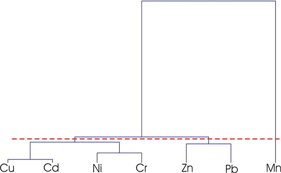
Fig. 5.
Dendrogram created for all bunkers using trace metals (TMs).
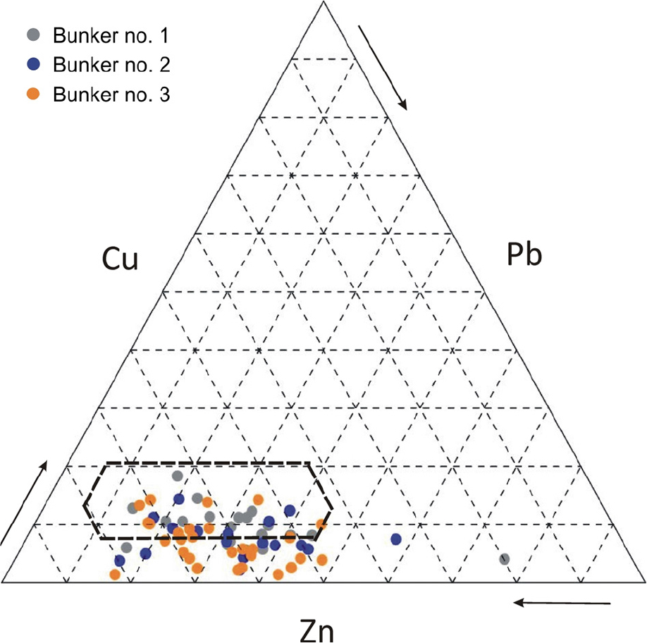
Fig. 6.
Ternary plot Cu, Pb and Zn (bunker No. 1 – grey points; bunker No. 2 – blue points and bunker No. 3 – orange points).
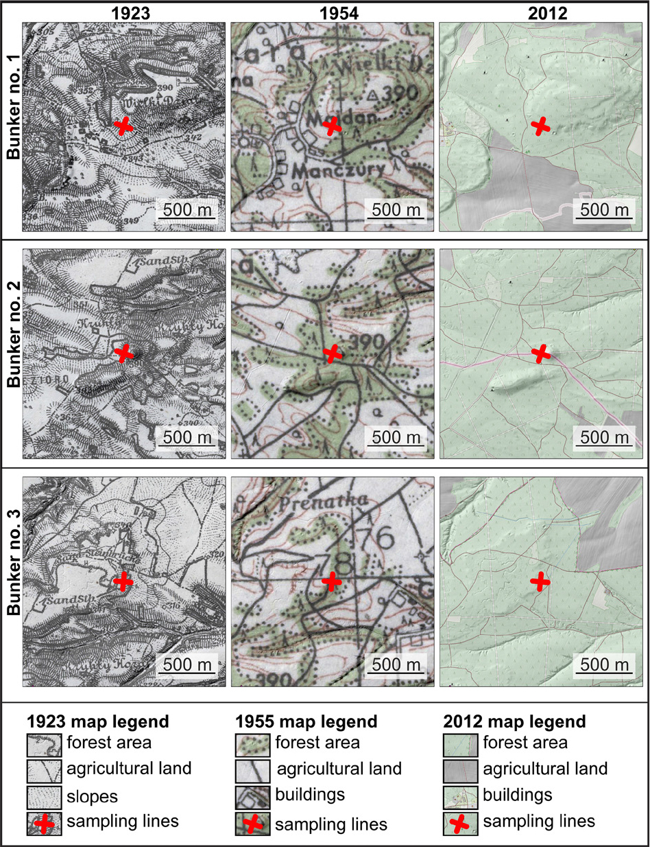
Fig. 7.
Land use changes within the surveyed military sites in 1923, 1954 and 2012 (background map source: WMS and WMTS viewing services, Central Office of Geodesy and Cartography, Poland).