

1. Introduction
Segmentation of brain tumors using magnetic resonance imaging (MRI) is an important aspect of clinical diagnosis, treatment planning and monitoring of disease progression. Radiotherapy planning, surgery, and treatment strategies need to be precise in sub regions of tumors, including the entire tumor, tumor core and enhancing tumor. Nevertheless, manual brain tumor segmentation is tedious, subjective, and prone to inter-observer variability, which has led to the development of automated and reliable brain tumor segmentation methods. In the last ten years, there has been a spectacular success of the use of deep learning-based approaches, especially convolutional neural networks (CNNs), in medical image segmentation. With their encoder-decoder design and skip connections which tend to combine low-level detail of the spatial features with higher-level semantic features, architectures such as U-Net and its variants have become standard baselines. Although CNN-based models have been quite successful, they have the perilous limitation of having local receptive fields that limit the extent to which they can capture long range dependencies and global relationships. This drawback is particularly problematic in brain tumor segmentation, where tumors differ greatly in shape, size, location and appearance and where tumor boundaries tend to be similar to the neighboring healthy tissues. Figure 1 shows the sub-regions that help healthcare professionals judge differences in a tumor and choose the best treatment approach to solve these problems, medical image analysis has recently seen the introduction of transformer-based architectures. Transformers, which were initially designed to work with natural languages, use self-attention to model global contextual relationships. Vision Transformers (ViTs) and their variants have demonstrated promising performance in allowing long-range feature interactions. Nevertheless, regular ViTs are computationally costly and need extensive training information, which is not feasible with high-resolution 3D medical images. In response to this, the Swin Transformer provides a more efficient alternative with shifted window-based self-attention hierarchy. The design enables the model to capture both the local and global contexts without expending too much computational complexity. As a result, medical image segmentation has been widely studied, with Swin Transformer-based models gaining growing popularity. Still, current Swin-based methods tend to not maintain fine-spatial resolution, particularly when small tumor objects are involved, and can exhibit inconsistency across features in multiscale fusion when coupled with encoder decoders. In this article, we present SwinNetPlus, a new hybrid deep learning model capable of combining the benefits of Swin Transformers and CNNs in the powerful segmentation of brain tumors in 3D MRI scans. The proposed model is aimed at overcoming the major issues of existing models, which include the problem of changes in scale, unclear delineation of tumors, and the visual resemblance of tumors and healthy tissues. The encoder-decoder model adopted by SwinNetPlus is capable of integrating a global contextual representation with high spatial localization. One of the biggest contributions of SwinNetPlus is the dedicated introduction of two new modules, namely the Spatial Local Attention Module (SLAM) and the Dense Cross-Multiplication Link (DCML). SLAM increases the sensitivity of the network to local spatial characteristics as it focuses on boundary and texture information, which are important in precise tumor delineation. This module allows the model to pay attention to minute changes that are likely to be missed by traditional attention systems. DCML, favors consistency in features and an overall healthy flow of information by blurring multiscale features through cross-multiplicative interactions, thus, minimizing noise and eliminating unhelpful activation. The SwinNetPlus encoder is designed based on Enhanced Local Self-Attention (ELSA) transformer blocks that enhance local feature extraction and maintain global contextual features. These features include channel squeeze-and-excitation blocks to re-calibrate channel-wise feature responses and improve the discriminative feature representation of various MRI modalities. Therefore, the proposed SwinNetPlus architecture is effective on the BraTS 2021 dataset that includes 1,251 multimodal 3D brain MRI scans. Experimental findings show that SwinNetPlus performs better than various state-of-the-art 3D segmentation algorithms with a Dice score of 92.69% and a Hausdorff distance of 5.34 mm. These findings indicate that the model is capable of splitting tumors in the brain even in difficult imaging conditions. In general, SwinNetPlus offers a powerful and efficient platform to segment brain tumors automatically, which has great potential to be applied in practice and contribute to the development of state-of-the-art medical image processing.
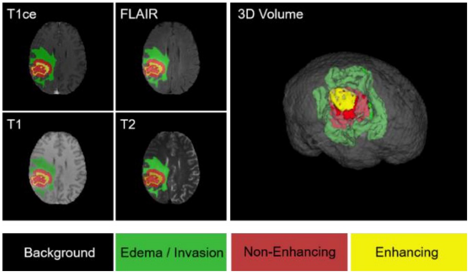
Figure 1.
Illustration depicting various sub-regions for brain tumor segmentation [1]
2. Related Work
The automated segmentation of brain tumors is a promising research topic because it has been found to be essential in clinical decision-making and treatment planning. First generation research used early computational methods used manual features and classical machine learning models. These methods, however were very sensitive to noise, changes in intensity and anatomical variability of the MRI scans. The introduction of deep learning in the field has superseded most traditional methods with data-driven ones as they are more effective at learning features.
2.1. CNN-Based Segmentation Techniques
Fully Convolutional Networks (FCNs) were a breakthrough in the field, because they allowed end-to-end semantic segmentation without fully connected layers [2]. U-Net (building on this concept) proposed a symmetric encoder-decoder network with skip connections, which maintain spatial resolution and learn high-level semantic features [3]. U-Net and its variants have emerged as hallmarks of biomedical image segmentation. Several variants include UNet++ [4], which added internal skip connections meaning the encoder and decoder features lessened the semantic disparity, leading to more accurate segmentation. In the case of volumetric medical data, 3D CNNs were designed to better utilize spatial continuity. The 3D U-Net was an extension of the U-Net framework to three dimensions and showed better results in volumetric segmentation tasks [5]. H-DenseUNet was a hybrid CNN architecture that used dense connectivity alongside encoder decoder architectures, and improved feature reuse and gradient flow [6]. Although effective, CNN based models have a small receptive field, which does not allow them to capture long range dependencies that are important in the process of contrasting tumors against visually similar normal tissues.
2.2. Transformer-Based Vision Models
Transformers, which were proposed as sequence models in natural language processing [7], were subsequently applied to visual tasks with the establishment of the Vision Transformer (ViT), which estimates the relationships globally via self-attention mechanisms [8]. Despite the excellent representational abilities of ViTs, the high cost of computation and the amount of data needed challenged the applicability to medical imaging. To address these drawbacks, hierarchical transformers like the Swin Transformer were proposed and utilized. These transformers use shifted window-based self-attention to balance both local and global context in an efficient way [9]. The Swin Transformer has since become a standard in image fusion models [10] as well as medical image segmentation models. SwinPA-Net [11] used multiscale feature pyramids to enhance the output of segmentation, whereas Swin-Unet used a U-Net-like design with pure transformer blocks [12]. Pure transformer designs, however, tend to have limited fine-grained localization of boundaries because they lack inductive bias on localizing spatial detail.
2.3. CNN-Transformer Hybrid Architectures
Hybrid architectures have been suggested in order to integrate the advantages of CNNs and transformers. TransUNet merged ViT encoders with CNN-based decoders showing better results than the pure CNN models [13]. UNETR used transformers as 3D medical image segmentation encoders, which utilized global context and volumetric consistency [14]. UNETR++ improved on this concept by making the 3D segmentation tasks more efficient and more accurate [15]. SwinBTS presented Swin Transformer blocks to analyze multiple modalities of MRI in the field of brain tumor segmentation, which brought positive results on the BraTS dataset [16]. NestedFormer was a proposed model of more attentive mechanisms that could be used to better integrate multimodal information by using modality [17]. Swin UNETR used Swin Transformer encoders with UNETR-style decoding to enhance the tumor boundary delineation [18]. Although these techniques enhanced contextual modeling, in many cases, they depended on global attention processes that can miss local structures important to accurately segmenting the boundaries of tumors.
2.4. Focusing Machinery and Character Strengthening
Both segmentation and robustness of segmentation have been highly exploited by attention-based feature refinement. The Squeeze-and-Excitation (SE) networks proposed channel-wise attention to refine the feature responses, and enhance the representational power with minimum overhead [19]. Enhanced Local Self-Attention (ELSA) was suggested to improve local context modeling in transformer architectures, fixing the loss of spatial detail using global attention [20]. Recent studies that incorporated ELSA in to Swin Transformers showed better performance in segmentation but still had the issue of multiscale feature consistency and noise suppression [21].
2.5. Research Gap
Although there have been major advancements, there are still a number of shortcomings in the methods for segmenting brain tumors. CNN based methods are not powerful in long-range dependency modeling, and transformer based methods usually do not have local sensitivity to features. Hybrid models enhance contextual awareness but often are affected by feature inconsistency when performing multiscale fusion and inadequate boundary refinement. In addition, Swin-based architectures do not sufficiently support the contemporaneous requirement of local spatial attention, strong interaction of multiscale features or noise reduction in complicated MRI scenarios. In order to close these gaps, a coherent framework that clearly improves local feature discrimination, dense and consistent interaction of features across scales, and effective global context integration is needed. The mentioned constraints drive the proposed SwinNetPlus, which use the Spatial Local Attention Module (SLAM) to model the fine-grained boundaries and a Dense Cross-Multiplication Link (DCML) to combine features and decrease noise.
3. Proposed Method
3.1. Overview
The proposed SwinNetPlus architecture is formed by an encoder and a decoder, as you can see in Figure 2. The main structure of the model uses the Swin Transformer to identify different levels of features from multimodal MRI scans. To make the feature representation stronger, we place the Enhanced Local Self-Attention (ELSA) blocks in the Swin Transformer. Additionally, the two new modules DCML and SLAM are included to help the model recognize both small-scale and wide-scale information. The input for SwinNetPlus is an MRI image X, where H, W, D and C denote the height, width, depth and number of modalities, respectively. The input is broken into separate patches and then goes through the transformer-based encoder. Swin Transformer blocks are used in the encoder and enhanced with ELSA modules to produce feature representations at different scales. The features from the encoder are passed through skip connections to the decoder path. The decoder contains a spatial Squeeze-and-Excitation (sSE) CNN module that combines multi-resolution features and outputs the final segmentation map. Using transformer-based encoding and convolution-based decoding, SwinNetPlus can use both global attention and precise local details.
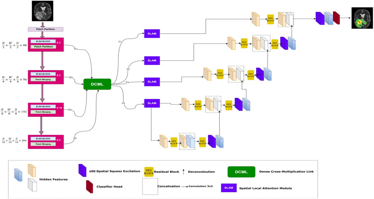
Figure 2.
SwinNetPlus Architecture
3.2. Swin Transformer Encoder
The proposed Swin Transformer-based encoder consists of four stages, and each stage is made up of two Swin Transformer blocks. Swin Transformer employs a special self-attention mechanism that helps improve speed and maintain the spatial arrangement. Window-based Multi-Head Self-Attention (W-MSA) units are followed by Shifted Window-based Multi-Head Self-Attention (SW-MSA) units in each layer, as shown in Figure 3(a). This progression help ensure that interactions between windows are effective without much extra cost in computation.
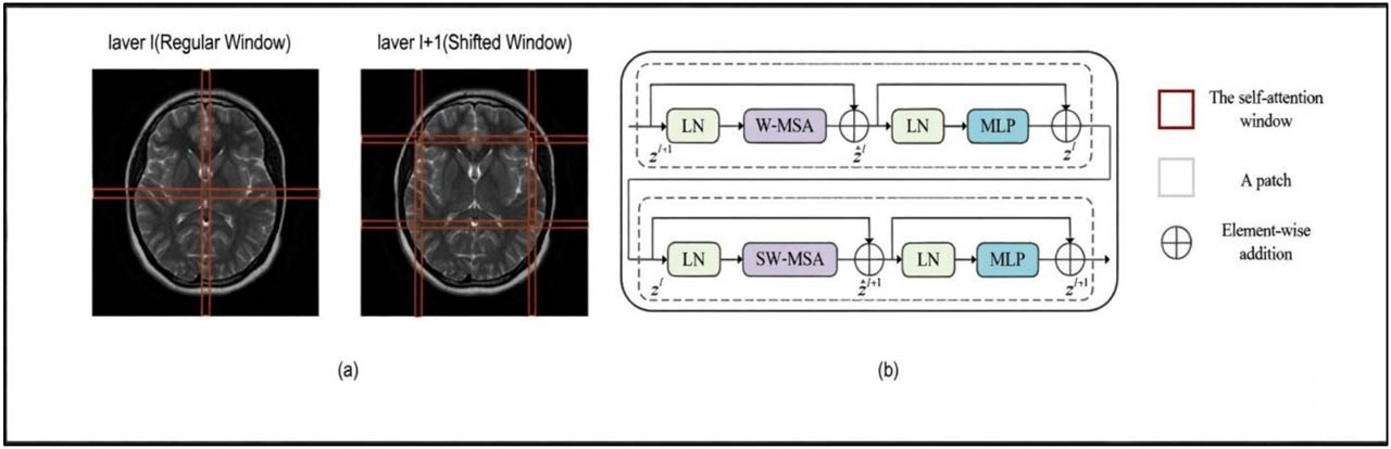
Figure 3.
The Swin Transformer architecture comprises distinct components. (a) Self-attention computations within adjacent layers l and l +1 utilize both regular and shifted windows. (b) Further insights into the intricacies of the Swin Transformer are provided
In the first three stages, ELSA blocks are included in the Swin Transformer. The blocks use Hadamard attention and ghost heads to impove local feature extraction by sharpening the attention inside the windows. This design makes it possible for the model to extract full and localized features from the given image. At this stage, windows are superimposed to improve the features even more. Self-attention is performed within every window helping to create rich contextual information with less computational cost. By sharing features, this strategy allows nearby windows to help to each other learn new features. Swin Transformer encodes multi-level features by gradually lowering the size of the input and adding more channels. Every time, a patch merging layer cuts the image’s size in half and increases the number of channels by two. At the beginning, C is set to 48 and then doubles at each level: (H/s) × (W/s) × C, (H/2s) × (W/2s) × 2C, (H/4s) × (W/4s) × 4C and (H/8s) × (W/8s) × 8C.
In this step, s is the patch size which is the number of patches taken from the input image that do not overlap. After the patches are flattened, they are sent through a linear embedding layer that projects them to C features and then the transformer blocks take over. It takes a lot of computing power for conventional transformers because they use global attention on all the tokens. The Swin Transformer addresses this by using a window-based system that both simplifies the model and keeps its representation strong. Both W-MSA and SW-MSA help windows share data and keep the system efficient. Because of its good balance between speed and effectiveness, the Swin Transformer is used in our SwinNetPlus model as the main component for extracting features from multimodal MRI data.
3.3. Enhanced Local Self Attention (ELSA)
Adding the ELSA block to the Swin Transformer gives it even greater ability to handle long-range connections. As shown in Figure 4, adding the ELSA block to the Swin Transformer’s structure allows it to better perform on dense prediction tasks [20]. The ELSA transformer block enhances the extraction of local features more than traditional Local Self-Attention (LSA) modules do, especially when it is used with dynamic filters in the Swin Transformer [3]. ELSA relies on Hadamard attention which uses Hadamard products to preserve high-level relationships and direct attention to nearby locations. Due to this, the model can now show relationships in space more clearly. Higher-order mappings, such as those utilized by Hadamard attention, are widely acknowledged to offer better feature fitting capabilities [3].
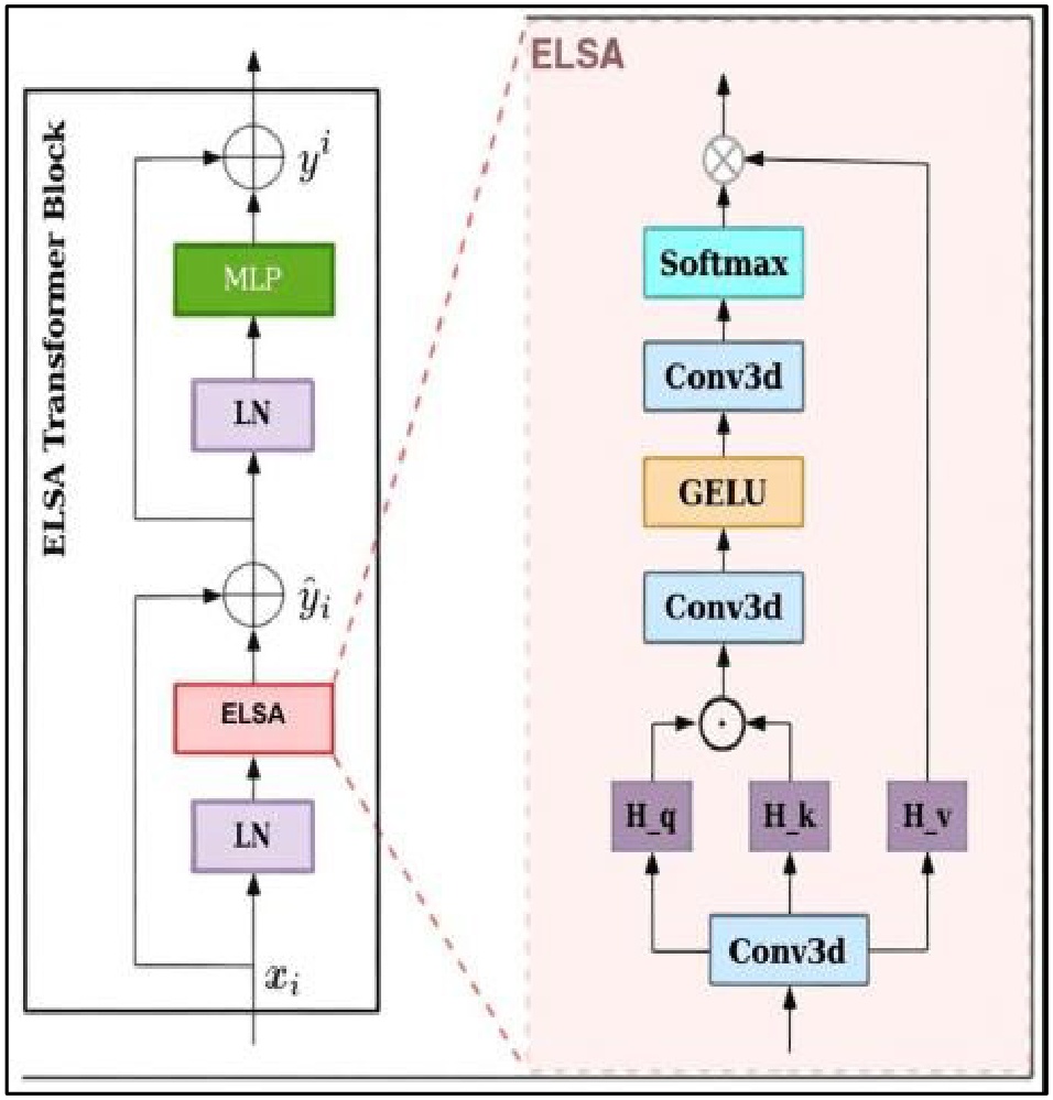
Figure 4.
Swin Transformer with ELSA Block [20]
For example, a study by Ronnnberger, Fischer, and Brox [3] demonstrates that Equation (1) defines a second-order attention mechanism, effectively mapping the input through a higher-dimensional space. This higher-order transformation allows for more expressive feature modeling. In contrast lower-order mappings, may result in reduced accuracy in complex tasks.
3.4. ELSA with Hadamard Attention
In this case, the input feature map is represented by xi, the convolution process is shown by f(xi), and the output feature map is yi. Because the second-order term qikj and the value vi are included, the self-attention structure in the Transformer represents the input xi in a third-order manner. This could be one of the reasons why the finished product has to be improved even more. ELSA with Hadamard attention [8], in which the Hadamard product is inserted as the second-order term between queries and keys, is one such approach. The following is an expression of Hadamard attention formulation (2):
The symbol ⊙ performs Hadamard multiplication on operations f(xi), which is a convolution while Hk, Hq, and Hv indicate feature maps extracted through the linear transformation input. The design of the ELSA Transformer module includes adding a duplicate multi-layer perceptron (MLP) module behind the attention structure and integrating it with the Transformer structure, while Figure 2 shows this implementation (as explained by Eq. (3)).
3.5. Addressing Shallow Feature Noise via the DCML Module
Brain tumor segmentation tasks aim to guide the network’s attention toward the relevant tumor regions. However, significant challenges arise due to variations in tumor size—particularly when tumors are very small—making accurate localization difficult. One of the key issues stems from the encoder’s progressive downsampling operations, which produce increasingly coarse feature representations. This process often leads to the loss or compression of crucial boundary information, thereby compromising segmentation accuracy.
A number of approaches have been suggested to address this problem. Using larger images as input allows one to create larger feature maps, which helps to keep more information about the image’s position. Yet, using this technique requires a lot more computing power. A further approach is to merge shallow and deep features, using the fine boundaries in the shallow layers, however, it is difficult to successfully combine these elements. Some fusion methods put in additional information that is not needed, as shallow feature maps keep a lot of background noise. But when feature fusion is involved, this noise can reduce the accuracy of segmentation. To handle this issue, we introduce the Dense Cross-Multiplication Link (DCML) module as seen in Figure 5. Subfigure 5(a) presents a simple type of skip connections that do not include fusion across scales. In subfigure 5(b), dense addition is used to add up the features from different scales. Subfigure 5(c) uses dense concatenation to combine the features by channel. In subfigure 5(d), the proposed DCML method is seen, using multiplicative fusion to add semantic information and reduce the influence of minor features. All models use Batch Normalization (BN) to help the training stay stable and make sure the features are always distributed evenly.
Because the DCML module brings together features of various scales, it helps produce more accurate and reliable segmentation, especially for small or uncertain targets in medical images. It merges feature maps from different scales which allows high-level information and low-level details to work together. By integrating features at different scales, the model can pay attention to both shallow and deep features. For example, at the fusion stage m, the output is calculated using Em (m=1,2,3,4) as seen in Eq.(4).
The feature transformation in the given context is g, which uses upsampling for resolution restoration and a 1×1 convolution for channel reduction. Three alternative fusion strategies and the multiplicative feature fusion approach are contrasted visually in Figure 5. Without feature fusion, Subfigure 5(a) uses the U-Net’s jump connection method, which introduces noise from shallow information and improves image segmentation only slightly.
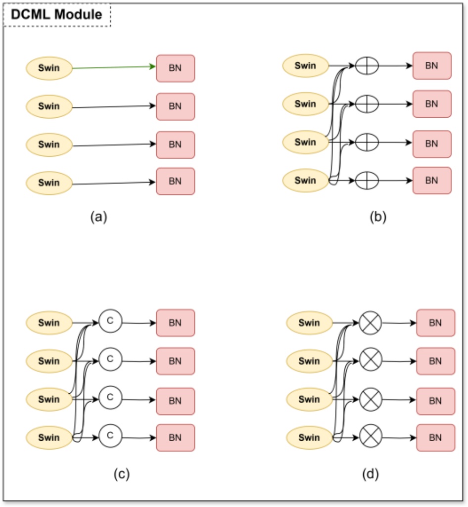
Figure 5.
DCML Module
In Subfigures 5(b) and (c), shallow and deep features are integrated by addition and concatenation fusion techniques, respectively. These two approaches, however, ignore the relationship between multiscale properties. The following equations can be used to express the three previously described methods:
The following equations can be used to explain the computations made when the neural network back propagates to determine the gradient:
Equations (8) and (9) demonstrate that the gradient of every branch does not depend on other branches and is not affected by the addition or concatenation of other branches. So, because each branch’s output does not influence the others, the network struggles to find connections between branches. Alternatively, with multiplication, the gradient of a branch can respond to changes in other branches, unlike with the initial technique. So, if one branch cannot combine the top features, multiplicative fusion will bring attention to the issue by creating a large gradient. Therefore, while training, the multiplication feature fusion approach creates strict limits on every branch helping each branch collect better features. Because of this connection between branches, each branch improves and the results are more precise.
3.6. Spatial Local Attention Module (SLAM)
Medical image segmentation models using deep learning often rely on spatial attention mechanisms such as the Spatial Local Attention Module (SLAM). SLAM is designed to help the model selectively focus on tumor-specific regions in brain MRI scans, thereby improving segmentation accuracy by enhancing the representation of clinically important spatial information.
The input to SLAM is a feature tensor of size C/N×H×W, where C is the number of channels, N is the number of samples, and H×W is the spatial dimensions. SLAM initially aggregates the spatial contextual information by summing corresponding activations across the feature maps, strengthening the relational understanding between different anatomical regions.
To obtain robust and discriminative spatial cues, SLAM employs two complementary pooling operations: Average Feature Extraction (AFE), which captures global contextual responses, and Maximum Feature Extraction (MFE), which preserves the most salient tumor-related activations. The pooled features are concatenated along the channel axis to generate a fused representation Se∈R2×H×W, enabling the module to encode both dominant and supporting spatial structures. A convolution operation is then applied to Se to learn an attention map Sconv∈R1×H×W, which assigns higher weights to tumor-relevant areas while suppressing less informative regions. This attention map is subsequently multiplied element-wise with the original input feature map to produce the spatially enhanced output Sact, which emphasizes pathological characteristics essential for accurate tumor delineation. During decoding, the SLAM output is fused with features from DCML and other decoder layers using skip connections and progressive upsampling operations. Bilinear interpolation followed by 3×3 convolutions refines structural boundaries, while a final 1×1 convolution restores the feature map dimension to align with the segmentation output space. By integrating localized attention into the decoding pathway, SLAM significantly improves the segmentation of whole tumor (WT), tumor core (TC), and enhancing tumor (ET) regions. In the final step (see Figure 6), the recovered features are passed through a spatial and channel Squeeze-and-Excitation (sSE) Block to refine segmentation accuracy. The sSE Block compresses the feature map U along the channel axis and excites spatially significant regions using a sigmoid activation function and a 1×1×1 convolution. This selective enhancement contributes significantly to fine-grained tumor segmentation.
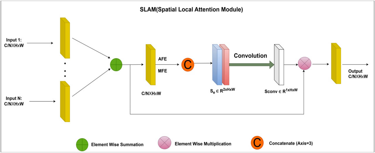
Figure 6.
The architecture of the SLAM module
Finally towards the end of the encoder pathway, upsampling, and adjustments to the channel count are made with 1x1 convolutions to push the feature map process in the prior stage back to the input image size. After that, as shown in Figure 7 the recovered features are enhanced by applying an sSE Block to give spatial and channel-wise excitation for image segmentation. A feature map U is compressed along channels and spatially excited by the sSE Block, which makes a major contribution to fine-grained image segmentation. A sigmoid activation function and a 1×1×1 convolution layer are used to calculate the final segmentation outputs.
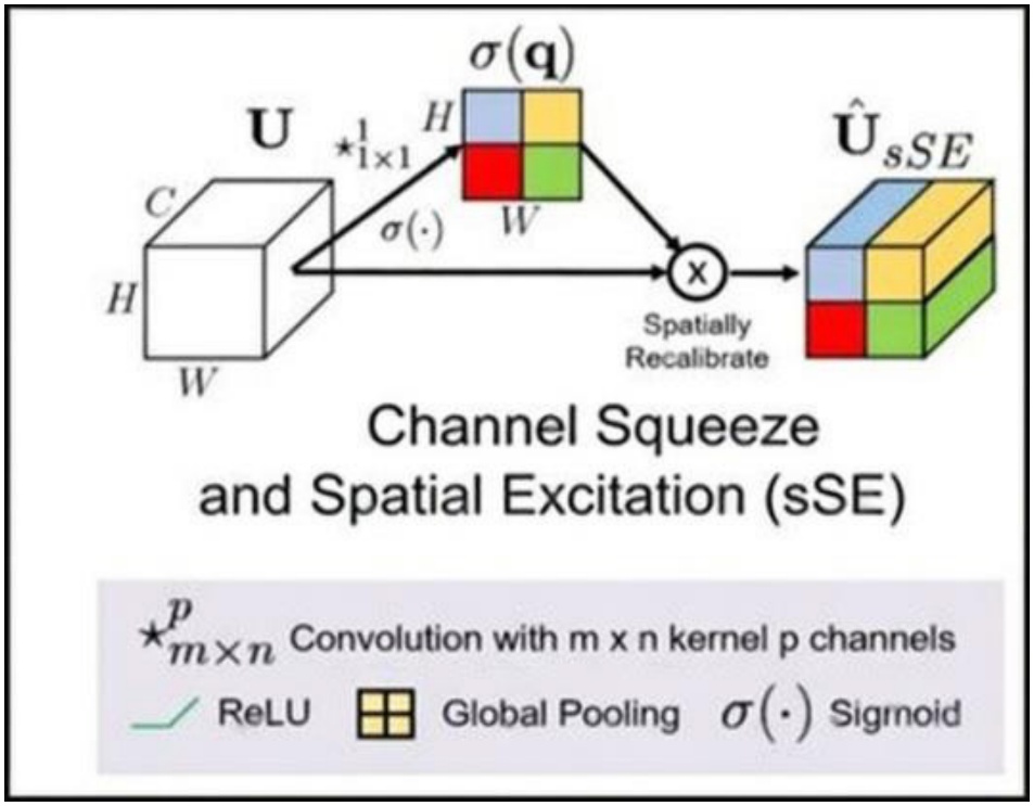
Figure 7.
Channel Squeeze and Spatial Excitation (sSE[21])
3.7. Loss Function
In medical image segmentation, disparities in lesion sizes and shapes, as well as unbalanced foreground-background distributions, are common issues. To overcome these problems, we propose a novel loss function that blends binary cross-entropy (BCE) loss (Equation 12) with dice loss (Equation 11). This combo approach increases the effectiveness of both model training and optimization. The formulation of this integrated loss function is described below:
In this case, y is the image’s actual label, p is the expected outcome, and ε is a parameter that is set to 1 for increased stability. Using this aggregated loss function enables the network to converge quickly and steadily, producing good results on a range of medical image datasets. Furthermore, we used this loss function in our comparative experiments for training all the systems under comparison for various segmentation tasks.
4. Experiments and Results
4.1. Dataset
We trained and validated our built model using the BraTS2021 dataset, which we acquired from the BraTS competition. This training dataset includes 1251 brain imaging cases with matching segmentation labels for each case (as seen in Figure 8). The four different 3D MRI modalities included in each case are T1-weighted (T1), T1-enhanced contrast (T1ce), T2-weighted (T2), and T2 fluid-attenuated inversion recovery (FLAIR). To attain a uniform isotropic resolution of 1 × 1 × 1 mm, the image dimensions for each modality are standardized to 240×240×155. They are then aligned, resampled, and skull-stripped.
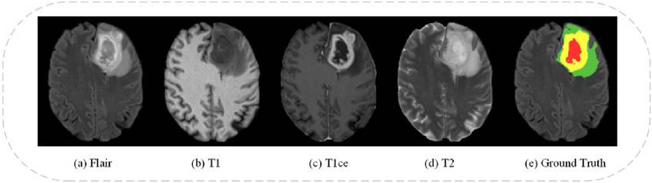
Figure 8.
Illustration depicting various modalities of BraTS 2021[1]
4.2. Assessment metrics
The 95% Hausdorff distance (HD) and the Dice score coefficient (DSC) are two metrics used to evaluate the precision of brain tumor segmentation. The mathematical formulae (13) and (14) provide the DSC and HD readings, respectively.
Gi and Pi stand for voxel I’s actual and expected values, respectively, and G′i and P′i for the sets of ground truth and predicted surface points. While the greatest Hausdorff Distance (or HD) is one thing, the 95th percentile of distances between border points in G′ and P′ is another. This measure is used to reduce the impact that a small number of outliers may have on the evaluation as a whole.
4.3. Results
We randomly partitioned the BraTS 2021 training dataset into training and validation subsets, consisting of 1,188 and 63 subjects, respectively. This partitioning was necessary because semantic segmentation labels for the official BraTS 2021 validation set are not publicly accessible. The results presented in Table 1 reflect the performance of our model on the internal validation set derived from the BraTS 2021 training data. We obtained an average Dice score of 92.69 percent and an average Hausdorff Distance (HD) of 5.34 mm for all three subregions of tumors. In particular, the Enhancing Tumor (ET), Tumor Core (TC) and Whole Tumor (WT) scored 90.12 percent, 94.19 percent and 93.77 percent on Dice and 7.32 mm, 4.40 mm and 4.31 mm on Hausdorff. Figure 9 shows the qualitative results of our method which prove its effectiveness. WT is shown in green and orange, TC in green and gray and ET in red in the annotations. The model clearly separates the tumor regions in the first three rows of Figure 9. Our method is shown to be correct and reliable in locating tumor areas. At the same time, the fourth row reveals that the model has challenges when trying to identify the exact regions of the tumors. This may happen because of different levels of intensity or the challenging structure of the tumor. These findings show that it is difficult to accurately identify tumors with unusual shapes or mixed features. Although there are some gaps, our model does well in most cases with exceptions present in brain tumor segmentation tasks. The last row highlights instances where segmentation could be improved.
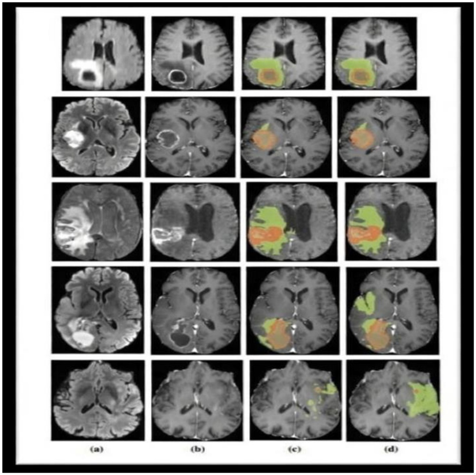
Figure 9.
Segmentation results of the proposed method: a. FLAIR, b. T1ce, c. proposed method, and d. ground truth segmentation
Table 1.
Summary of Key Related Works and Limitations
| Author(s) | Method | Key Contributione | Limitation |
|---|---|---|---|
| Long et al. [2] | FCN | End-to-end semantic segmentation | Poor boundary localization |
| Ronneberger et al. [3] | U-Net | Encoder–decoder with skip connections | Limited global context |
| Zhou et al. [4] | UNet++ | Nested skip connections | Increased complexity |
| Çiçek et al. [5] | 3D U-Net | Volumetric segmentation | High memory usage |
| Dosovitskiy et al. [8] | ViT | Global self-attention | Computationally expensive |
| Liu et al. [9] | Swin Transformer | Efficient hierarchical attention | Weak local boundary sensitivity |
| Chen et al. [13] | TransUNet | Hybrid CNN–Transformer | Feature inconsistency |
| Hatamizadeh et al. [14] | UNETR | Transformer encoder for 3D data | Requires large datasets |
| Jiang et al. [16] | SwinBTS | Swin-based brain tumor segmentation | Limited local attention |
| Ghazouani et al. [21] | Swin + ELSA | Enhanced local attention | Inadequate multiscale fusion |
| Xing et al. [17] | NestedFormer | Modality-aware transformer | High computational cost |
The segmentation performance on the BraTs 2021 validation dataset is compared with that of six state-of-the‐art methods in Table 2. To measure performance, Dice Score (percent) and 95 percent Hausdorff Distance (mm) are used for ET, TC and WT. When compared to other models, our method attains the highest average Dice accuracy (92.69 percent) and the best Hausdorff distance (5.34 mm). It is most accurate for WT (93.77 percent) and TC (94.19 percent). The robustness and effectiveness of our model in these results correctly splitting up different parts of tumors in MRI images.
Table 2.
Segmentation outcomes observed on the BraTS 2021 validation dataset
| Method | Dice Score (%) | 95% Hausdorff Dist. (mm) | ||||||
|---|---|---|---|---|---|---|---|---|
| ET | TC | WT | AVG. | ET | TC | WT | AVG. | |
| UNETR[14] | 58.5 | 76.1 | 78.9 | 71.16 | 9.35 | 8.84 | 8.26 | 8.81 |
| 3DUNet[5] | 83.93 | 85.11 | 89.15 | 85.97 | 4.73 | 11.92 | 12.26 | 10.26 |
| NestedFormer[17] | 80 | 86.4 | 92 | 86.13 | 5.26 | 5.31 | 4.56 | 5.04 |
| SwinBTS[16] | 83.21 | 84.75 | 91.83 | 86.59 | 16.03 | 15.51 | 3.65 | 8.54 |
| SegTransVAE[22] | 85.48 | 90.52 | 92.6 | 89.53 | 2.89 | 3.57 | 5.84 | 4.1 |
| Swin UNETR[18] | 85.8 | 88.5 | 92.6 | 88.96 | 6.01 | 3.77 | 5.83 | 5.2 |
| Our Method | 90.12 | 94.19 | 93.77 | 92.69 | 7.32 | 4.4 | 4.31 | 5.34 |
4.4. Ablation Study
To evaluate the contribution of each component within our proposed SwinNetPlus architecture, we conducted a detailed ablation study on the BraTS 2021 validation dataset. Specifically, we assessed the impact of the Dense Cross-Multiplication Link (DCML), the Spatial Local Attention Module (SLAM), and the multiplicative fusion strategy. Table 2 summarizes the performance of different ablated variants using Dice Score (percent) and 95 percent Hausdorff Distance (mm).
Table 3.
Ablation study of SwinNetPlus on the BraTS 2021 validation dataset
| Model Variant | DCML | SLAM | Mult. Fusion | Dice Score (AVG) ↑ | 95% HD (AVG) ↓ |
|---|---|---|---|---|---|
| Baseline ( without DCML/SLAM) | ✗ | ✗ | ✗ | 87.15 | 6.93 |
| Baseline + DCML | ✓ | ✗ | ✓ | 88.76 | 6.15 |
| Baseline + SLAM | ✗ | ✓ | ✗ | 89.21 | 5.94 |
| Baseline + DCML + SLAM (Additive Fusion) | ✓ | ✓ | ✗ | 90.03 | 5.59 |
| Full Model (SwinNetPlus) | ✓ | ✓ | ✓ | 92.69 | 5.34 |
In Fig 10 visual comparison of the ablation study highlights the progressive improvement in model performance with the addition of DCML, SLAM, and Multiscale Fusion. The Dice Score (AVG) increases steadily from 87.15% in the baseline model to 92.69% in the full SwinNetPlus model, indicating better segmentation accuracy. Simultaneously, the 95% Hausdorff Distance (AVG) decreases from 6.93 mm to 5.34 mm, demonstrating enhanced boundary precision. These results confirm that each added component contributes to performance gains, with the combined use of DCML, SLAM, and Multiscale Fusion achieving the most accurate and precise segmentation on the BraTS 2021 validation dataset.
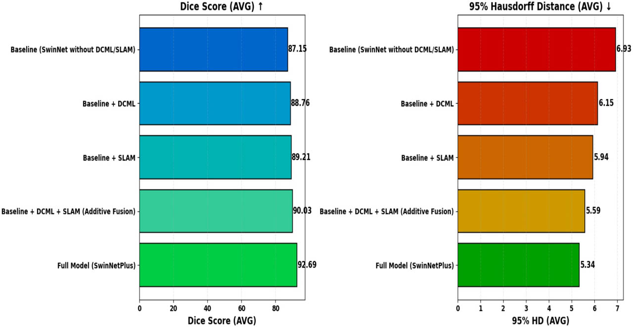
Figure 10.
Ablation Study Results of SwinNetPlus on the BraTS 2021 Validation Dataset
5. Discussion
The results obtained from the evaluation of SwinNetPlus on the BraTS 2021 dataset demonstrate the model’s effectiveness in addressing the primary challenges of brain tumor segmentation, such as lesion heterogeneity, varying tumor sizes, and the need for accurate boundary delineation. Compared to other state-of-the-art methods like UNETR, 3DUNet, and Swin UNETR, SwinNetPlus consistently achieved superior performance across all key metrics, including Dice score and Hausdorff Distance. This improvement can be attributed to the synergy between the convolutional backbone and the hierarchical attention mechanisms of the Swin Transformer, which together facilitate comprehensive global and local feature extraction. The inclusion of ELSA transformer blocks within the encoder played a crucial role in enhancing long-range dependency modeling while preserving fine-grained local details, a limitation of conventional CNN-based models. Moreover, the DCML module effectively addressed the problem of feature degradation during fusion by leveraging multiplicative interactions that preserve semantic richness while suppressing noise. Similarly, the SLAM allowed the network to focus selectively on critical spatial regions, further refining the segmentation quality, particularly along tumor boundaries. Despite the strong performance, certain limitations were observed. In some complex cases, particularly in instances with highly irregular tumor morphologies or low contrast between tumor and healthy tissue, the model exhibited reduced segmentation precision. This suggests that even advanced attention modules may struggle to generalize across all imaging conditions, highlighting the need for further enhancements in feature sensitivity and robustness. Additionally, while the current architecture is computationally efficient compared to many 3D models, inference time and resource utilization remain important considerations for clinical deployment. Future optimization of the model for real-time processing and integration into diagnostic workflows would be essential for translational impact. Overall, the proposed SwinNetPlus model represents a significant advancement in automated brain tumor segmentation. The combination of transformer-based attention, dense feature fusion, and spatial refinement modules contributes to improved diagnostic accuracy, supporting the model’s potential application in clinical decision-making. Future directions should explore the generalizability of this architecture to other medical segmentation tasks, as well as investigate architectural modifications and novel attention strategies to further boost performance and interpretability.
6. Conclusion and future work
In summary, this study introduces SwinNetPlus, an innovative deep learning framework designed to accurately segment brain tumors from MRI scans. By effectively integrating Convolutional Neural Networks (CNNs) with Swin Transformers, and incorporating advanced modules such as the Dense Cross-Multiplication Link (DCML) and the Spatial Local Attention Module (SLAM), the architecture demonstrates a strong ability to capture complex spatial and semantic features. The SLAM enhances the model’s attention to tumor-relevant regions, enabling finer discrimination of subtle variations, while the DCML module reduces background noise and improves multiscale feature fusion through an efficient multiplicative strategy. The use of ELSA transformer blocks within the encoder strengthens long-range dependency modeling and detailed local feature extraction, further refined by channel squeeze and spatial excitation blocks for enriched spatial and channel-wise representations. Evaluated on 1,251 annotated MRI volumes from the BraTS 2021 dataset, SwinNetPlus achieved an outstanding average Dice score of 92.69 percent and a Hausdorff distance of 5.34 mm, outperforming several state-of-the-art 3D segmentation models. These results confirm the effectiveness and robustness of SwinNetPlus in handling tumor heterogeneity and complex visual features. This work not only contributes a reliable method for brain tumor segmentation but also lays the foundation for future advancements in medical image analysis. Future research could explore expanding SwinNetPlus to segment other types of tumors or pathologies, as well as enhancing its performance through the integration of novel attention mechanisms, fusion strategies, or transformer architectures, thereby pushing the boundaries of automated medical diagnosis.