

1. Introduction
The aerial manipulator is a new type of aerial system that can both fly and physically interact with the world. Aerial robots have attracted much interest for their increased mobility compared to ground robots, as they are not restricted by terrain and can navigate in hard-to-access locations [1]. These systems offer solutions in environments that can be too dangerous for a human operator, and are used in diverse fields like inspection, transportation, architecture, building, and construction, as well as in military applications.
Nevertheless, the integration of a robotic arm with a floating base presents significant control difficulties. The system is subject to complex, time-varying dynamics coupling that results in strong nonlinearities. The motion of the manipulator and the interaction with varying payload continuously alter the system’s inertia tensor and shift the center of mass (CoM) during flight. Consequently, achieving robustly stable and precise control remains a complex problem.
The current control literature is full of different control methods for those systems that have been proposed to manage the coupled dynamics, including nonlinear, adaptive controllers and sophisticated compensation schemes. Despite these advances, existing control systems are still facing some limitations. To achieve robust stability, many designs including robust optimal methods like the classic nonlinear H∞ controller [2] — rely on explicit, continuous real-time calculation and compensation for the reaction forces induced by the robotic arm [3, 4]. Model-based solutions, derived from advanced techniques using numerical methods for dynamic compensation [5], increase computational cost and restrict the performance of those platforms [6]. Complex solutions — such as combining sliding mode control with adaptive laws and disturbance observers for simultaneous internal and external disturbance compensation [7, 8], or adaptive control methods combined with neural networks to manage high modeling error [8, 9] — are promising, but result in a large computational burden that can challenge a system’s stability during fast aerial manipulation maneuvers.
Control stability is often dependent on strictly-defined mechanical parameters. For example, stability conditions often rely on critical assumptions, like keeping the mass of the manipulator sufficiently small with respect to the aerial vehicle [4] or requiring complex algorithms to estimate time-varying inertia when manipulating objects [10]. These inherent structures are not impervious to the changes introduced by grasping different payloads [8, 11]. While robust stability can be analytically proved using complex frameworks like nested saturation control (achieving input-to-state stability) [3, 4], these systems are designed with controller structures that are difficult to tune across significantly varying flight conditions.
Based on preceding analysis, this study’s central research problem involves the trade-off between the high computational cost of real-time nonlinear compensation and the need for robust stability during fast maneuvers with varying payloads. Though current control methods for aerial manipulation can achieve stability, they typically rely on real-time calculations that create a significant computational burden, or lack the necessary robustness to handle rapid payload changes and fast maneuvers simultaneously.
To address this problem, the research objectives are as follows:
i) To minimize the real-time computational cost associated with nonlinear dynamic compensation.
ii) To enhance the adaptability of the control system to rapid shifts in payload characteristics and system inertia during fast maneuvers.
iii) To guarantee high-precision trajectory tracking and robust stability throughout the whole operational envelope.
The proposed solution is based on shifting the computational complexity to the pre-flight phase. By employing an inverse dynamics linearization [12] based on fixed, pre-computed nominal models, the complex nonlinear system can be transformed into a simple linear system with residual nonlinearities captured as bounded uncertainties. Those structured uncertainties are quantified using the Linear Fractional Transformation (LFT) framework [13]. The entire configuration space, including the manipulator state, the payload mass and the object dimensions, is divided into clusters using the K-Means algorithm, optimized via the Elbow Method [14]. For each local region, a PD controller is designed, and its gains are tuned using a multi-objective GA [15]. The reward function is tasked with minimizing the tracking error and the control effort, while maximizing the local robust stability margin using the Small Gain Theorem [13]. This method yields a control system that can tolerate grasping of various payloads in the defined range of object masses and dimensions.
2. System Dynamics
The aerial platform consists of a quadrotor base carrying a 2-DOF manipulator with two revolute joints, as depicted in Fig. 1. The kinematic description of the system is based on two coordinate systems, {I} inertial frame, and {B} body-fixed frame, aligned with the principal axes of inertia. The transition from {I} to {B} is given by the orthogonal rotation matrix constructed from the UAV’s Euler angles in the ZYX convention. The system state is defined using a generalized coordinate vector q∈R6, which consists of UAV’s height z in {I}, its attitude vector (roll, pitch, yaw) Ω=[ϕ,θ,ψ]T in {B}, and the manipulator’s joint angles ϒ = [ε1, ε2]T:
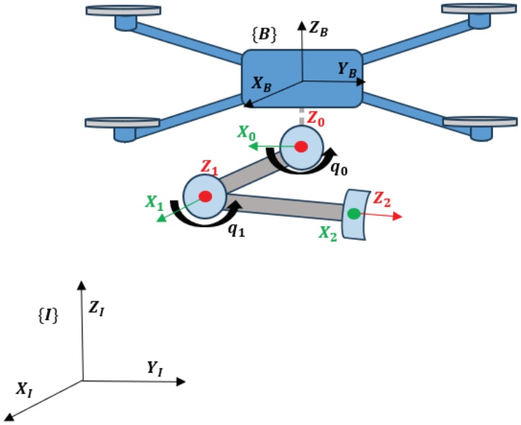
Figure 1.
UAV manipulator system
Unlike conventional UAVs, the dynamics of an aerial manipulator are intrinsically coupled to the arm’s motion, which displaces the CoM and alters the vehicle’s inertia tensor during the flight. The inputs driving the system are denoted as τ and combine the quadrotor’s aerodynamics with the servo torques:
where TΣ represents the collective thrust of the four rotors: where each i-th rotor generates a thrust Ti that is proportional to the square of angular velocity of rotors σi (i.e. ) and acts along the body-fixed axis ZB [16, 17]. The τϕ,τθ,τψ are the quadrotor torques, and τj1,τj2 are the torques of each joint of the manipulator. The thrust-to-torque mapping for the quadrotor can be expressed using the four-dimensional vector of thrusts Ti, (T̅UAV = [T1,T2,T3,T4]T), as well as the quadrotor configuration matrix BUAV:Given the needed controls TΣ and τ, the equation (4) allows for the computation of the required thrusts Ti (or, which is equivalent, the velocities σi) of the rotors. The system’s torque-to-input mapping can be described as:
where T̅SYS is the combined vector of the quadrotor motor’s thrusts and the manipulator joint torques. BSYS for the X configuration quadrotor with a 2-DOF robotic arm will have the form: where L is the length of the quadrotor arms, and kψ(kψ > 0) is the drag coefficient.The equations of motion of the system are derived using the Euler-Lagrange method [18], and have the standard form:
where M(q) is R6×6 symmetric, positive-definite inertia matrix, C(q,q̇) contains Coriolis and centrifugal terms, G(q) is the gravity vector, and τD is the disturbance force.To facilitate the control design, the Coriolis, centrifugal, gravitational and disturbance terms are combined into a single nonlinear vector N(q,q̇). Thus, equation (6) can be rewritten as
This equation is linear in the control τ, and has full rank M(q), which can be inverted for any valid configuration. Taking the control τ as a function of the manipulator states in the form:
leads to the system described by where y represents a virtual input vector: where r is the reference component [12, 19].This ideal linearization approach relies on the exact cancellation of nonlinearities in the system equations of motion. Its practical implementation requires consideration of various sources of uncertainty, including modeling errors, unknown payloads, and computation errors [20]. It also requires online computation of the exact time-varying M(q) and N(q,q̇), which is computationally expensive, impractical, and in some cases impossible for real-time aerial manipulation tasks. To overcome this, we propose using an offline computed fixed nominal model in the inverse dynamics controller (Fig. 2):
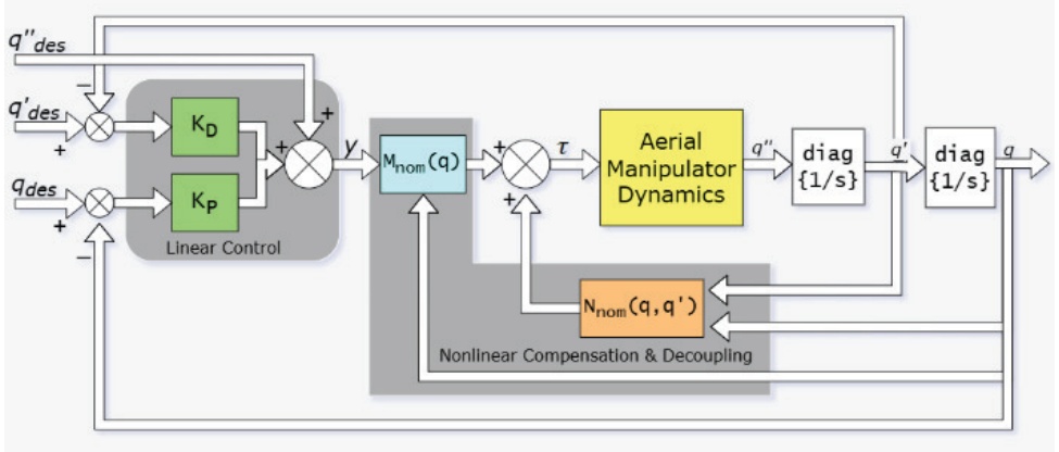
Figure 2.
Block diagram of the UAV manipulator system
This approach does not result in perfect cancellation of nonlinearities. Instead, applying (11) to the actual plant (7) results in a perturbed linear system. The difference between the fixed nominal model and the actual varying dynamics is isolated into structured uncertainty blocks. The system dynamics become:
where Δm, Δa are multiplicative and additive uncertainties:This formulation, shown in Fig. 3, allows us to treat the nonlinear complex aerial manipulator dynamics as a linear plant subjected to bounded perturbations that can be managed using robust control techniques.
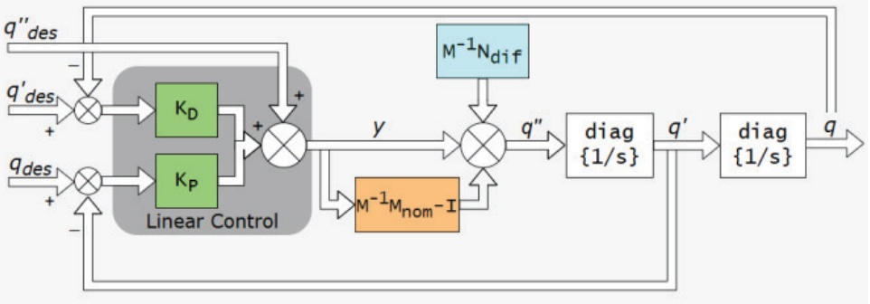
Figure 3.
Block diagram of the linearized system
The robust control input τ for the resulting system is expressed by:
where q̆ and q̐ are the tracking error and differential error terms.The robust stability of this control law against the uncertainties Δm and Δa is assessed through the μ-analysis and Small Gain procedure, as detailed in the next section.
3. Control System Design
The dynamic model derived in the previous section, particularly the feedback-linearized form in Eq. (12), isolates the system’s complex, time-varying, and payload-dependent dynamics into a structured uncertainty term: Δ = diag(Δm, Δa). For a global controller, the bounds on this uncertainty must encompass all possible manipulator configurations, velocities, and payload properties. Such a global bound is necessarily large, forcing a monolithic robust controller to be highly conservative. This severely degrades tracking performance and agility.
In this paper, a hybrid gain-scheduling framework is introduced to minimize the uncertainty bounds. The main strategy is to partition the system’s operating space into a finite K-number of smaller, dynamically-similar regions. If a dedicated controller is designed for each region, it is only necessary to guarantee stability against much smaller local uncertainty bounds, enabling high-performance control in every region.
3.1. Dynamic-Based State Space Clustering
To avoid the conservatism of a single robust controller, a comprehensive sampling space was defined that includes not only the manipulator kinematics, but also the full range of expected payload masses and object dimensions. The dataset, generated by sampling the manipulator’s kinematics and potential payload characteristics, is then subjected to unsupervised learning. The K-Means algorithm is employed to minimize the within-cluster variance of the dynamic parameters.
An important design parameter is the cluster cardinality K. Rather than arbitrarily selecting this value, the distortion curve is analyzed, plotting the within-cluster variance against an increasing number of centroids. By identifying the point of rate decrease — the geometric “elbow” of the curve — the optimal K number is determined, balancing model fidelity against controller complexity. This granularity ensures that within any specific cluster k, the deviation between the local nominal model and the actual dynamics remains within the predictable bounds required for robust stability synthesis. The distortion curve for the system is shown in Fig. 4, which represents the Sum of Squared Errors (SSE) against the number of clusters.
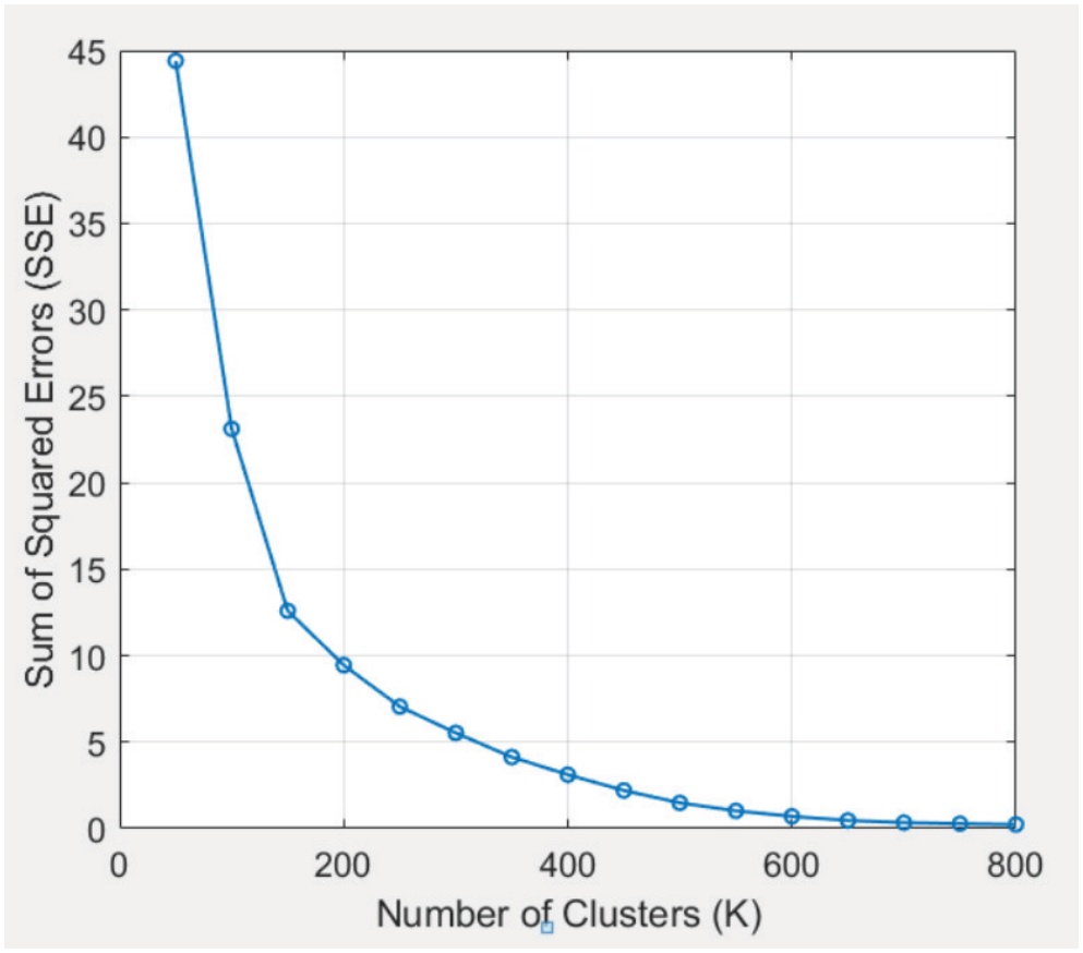
Figure 4.
Elbow method for optimal K
3.2. Robust Controller Synthesis
For each of the K regions, a dedicated robust controller is designed. The system, linearized by approximate inverse dynamics, is analyzed using the LFT framework, as shown in Fig. 5. This structure isolates the nominal plant P(s) from the local, bounded uncertainty .
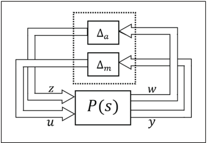
Figure 5.
LFT model of the system
The interconnection matrix G(s) maps the uncertainty blocks (y from Δm, w from Δa) to their respective inputs (y, z) through the nominal closed-loop system. For the 6-DOF system under consideration, with a diagonal plant and a diagonal PD controller K(s) = diag{K1 (s), … , K6 (s)}, where each , and where T is the time constant for the derivative filter, interconnection matrix G(s) is a 12 × 12 block matrix given by:
According to the Small Gain Theorem, robust stability for cluster k is guaranteed if the supremum of the structured singular value μΔ(P(jw)) is less than 1 for all frequencies w [13]:
where Ck is the local controller for cluster k. This condition can be expressed as ensuring the robust stability margin, βk = 1/μΔk, is greater than 1.Calculating the optimal feedback and that simultaneously satisfy the Small Gain condition βk > 1 and minimize tracking error is a non-convex optimization problem. To navigate this complex search space, a GA is employed to evolve a population of candidate controllers for each cluster. The fitness of each candidate solution is evaluated using a composite cost function that penalizes instability while rewarding precision. The evaluation criteria J balances 3 objectives:
where α1, α2, α3 are tuning weights. The first term minimizes the Root Mean Square Error (RMSE) of the step response, and the second term penalizes excessive control effort. The third term returns zero if the stability margin βk > 1, but applies a heavy penalty if the robust stability constraint is violated. Consequently, the optimization process selects a set of controller parameters that maximize precision without compromising the system’s stability margins. As can be observed from the relationship between the linearized dynamics (9) and the control law (10), the selection of positive-definite gain matrices ensures the asymptotic convergence of the tracking error to zero. This structure guarantees that the system accurately follows the desired trajectory, even when subjected to the bounded model uncertainties defined in (12).3.3. Gain-Scheduling Specification
The gain-scheduling framework functions as an adaptive mechanism that bridges real-time system dynamics and a library of robust controllers. During operation, the system calculates the Euclidean distance between the current dynamic state and the pre-computed operating points, or cluster centroids, which represent the partitioned workspace. By identifying the most relevant clusters in this space, the system retrieves the corresponding control gains that were specifically optimized during the offline tuning phase.
4. Simulation and Results
A series of simulations were conducted to validate the performance and robustness of the proposed control framework. The primary goal of the simulations was to demonstrate that the offline-tuned controller could robustly manage the dynamic variations introduced by rapid manipulator motion and the need to grasp a variety of payloads.
4.1. Simulation Setup
Simulations were conducted in the MATLAB software to validate the performance and robustness of the UAV manipulator system. The configuration space was sampled by focusing on the dominant variables: the manipulator joint angles, the payload mass, and the payload dimensions. The grid of manipulator positions was combined with a set of payload masses, along with three distinct object dimension sets (small, medium, and big). For each combination, a set of five fast velocity vectors (up to π/2 rad/s) were applied to capture the full dynamics, including Coriolis and Gravitational effects.
This process generated a comprehensive dataset of ∼30,000 valid dynamic samples di = [M, N]. The K-Means algorithm, using K = 300 (determined from the Elbow Method, Fig. 4), was used to partition this data, yielding 300 local nominal models .
The 99th percentile H∞ of the local uncertainty was calculated for each cluster. This resulted in significantly small bounds for both multiplicative ( ) and additive ( ) uncertainties (Fig. 6), which were then used as constraints for the controller synthesis.
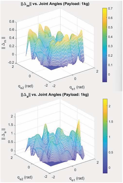
Figure 6.
Uncertainty norms in clusters
For each of the K = 300 clusters, a local diagonal PD controller was tuned, using the GA as described in the previous section.
The dynamic performance of the proposed system depends on the behavior of the entire setup, including the masses and dimensions of the UAV and manipulator. The physical parameters used in the simulations are summarized in Table 1.
4.2. Robust Stability Validation
The first validation test was conducted to confirm that the GA successfully synthesized controllers that meet the robust stability conditions. The robust stability margin, βk = 1/μΔk, was calculated using the final tuned controller in each of the 300 clusters. As shown in Fig. 7, the stability margin for all 300 clusters is greater than the robust stability boundary of β = 1.
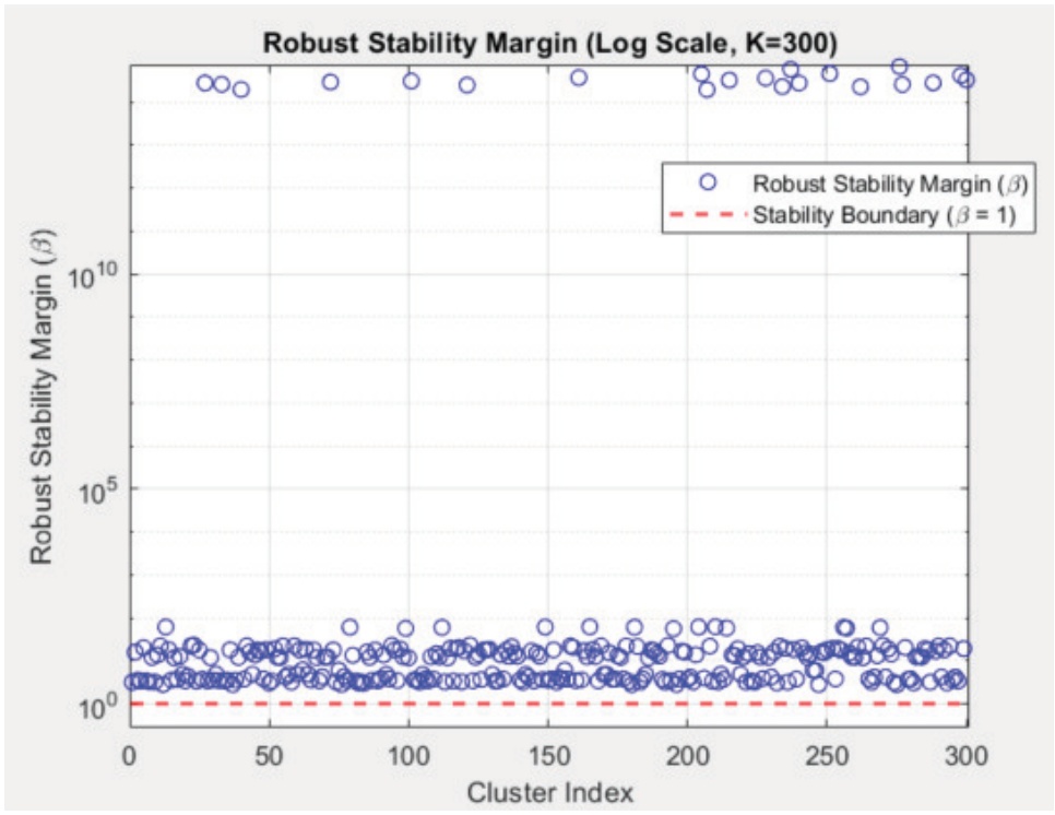
Figure 7.
Robust stability margin (β) on a logarithmic scale
This result confirmed that the offline GA tuning, constrained by the local bounds, successfully generated a set of controllers that are guaranteed to be robustly stable within their respective operating regions.
The second simulation was implemented to validate the adaptability and precision of the control framework when confronted with the simultaneous changes in both manipulator configuration and payload properties. This simulation was executed over a 30-second span, forcing the system through critical operational states. The UAV’s translational and attitude states were commanded to hold a still position of Z = 1m and ϕ, θ, ψ = 0, while manipulator joints were commanded to perform a sinusoidal tracking motion from −π/2 to π/2 radians, actively switching the payload every 10 seconds to stress the controller’s adaptability. The payload characteristics and corresponding grasping times are given below in Table 2.
Table 2.
Payload characteristics
| Object | Time | Mass (kg) | Dimensions (m) |
|---|---|---|---|
| Small | 0-10 sec | 0.1 | 0.1, 0.02, 0.02 |
| Medium | 10-20 sec | 0.5 | 0.4, 0.05, 0.05 |
| Big | 20-30 sec | 1 | 0.6, 0.08, 0.08 |
The resulting plots are depicted in Fig. 8. The plots show that the actual trajectory remains tightly coupled with the desired trajectory for all controlled states. Only minimal tracking errors were observed during the manipulation of the biggest payload configuration, and these deviations were quantitatively negligible.
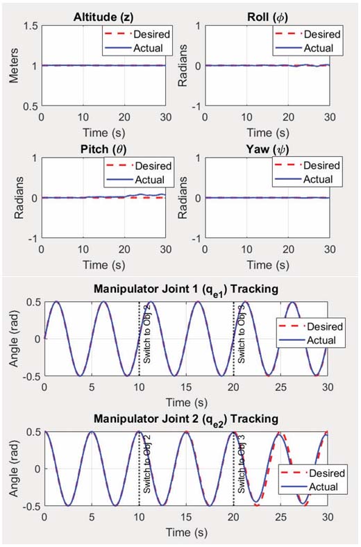
Figure 8.
Trajectory tracking of the system
Gain switching was logged along the simulations to analyze the control stability at transition points. To mitigate the potential for abrupt control actions, the gain interpolation technique was used to ensure a smooth transition between scheduled gains. Instead of selecting a single best controller, this method blends the control laws from multiple adjacent clusters. Using the k-nearest neighbors algorithm, the system identifies the four closest cluster centroids to the current dynamic state. This provides a set of indices for the four most relevant local controllers. For each of the neighboring clusters, the weight component wi is calculated based on its Euclidean distance Di from the current state. The weight is computed as the inverse of the distance, with a small ε added to avoid division by zero
The weights are then normalized to sum to one, esuring a stable weighted average:
The resulting gain-switch plot is presented in Fig. 9. As a result, a total of 176 gain switches occurred, with 48 unique cluster gains used, indicating continuous adaptation.
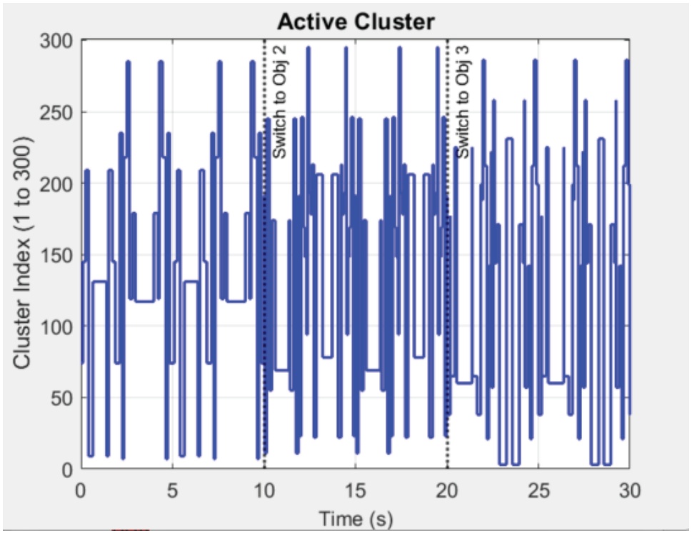
Figure 9.
Active cluster index over time
The integrated gain interpolation successfully mitigated the discontinuities of hard switching. This is quantitatively supported by the RMSE plot in Fig. 10, which confirms that the smooth switching mechanism helped maintain a consistently low tracking error across the entire mission, even when controlling the system under the biggest payload (Obj. 3).
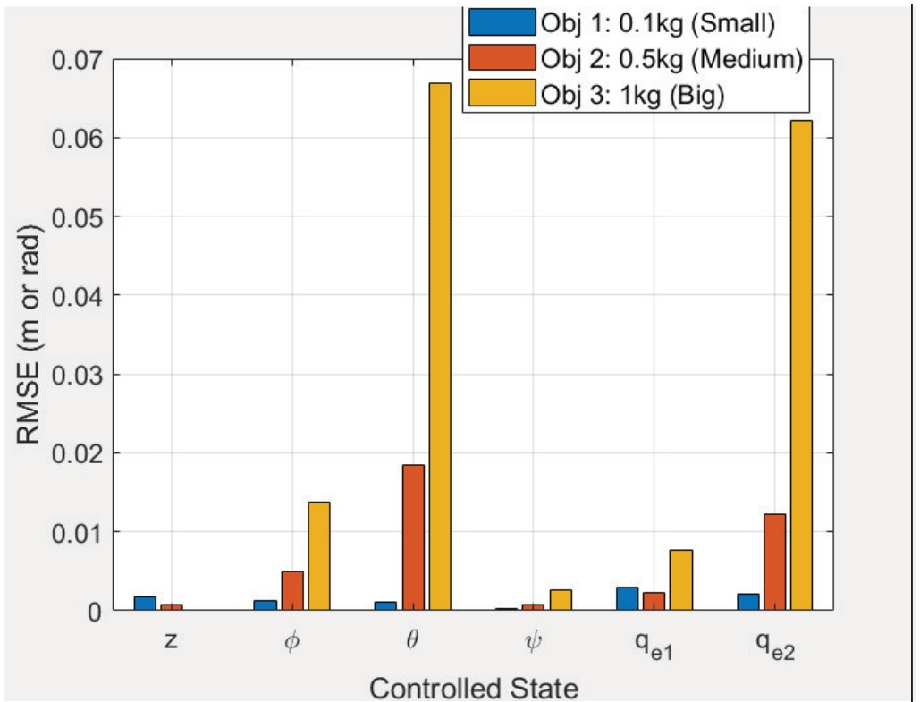
Figure 10.
RMSE by state
5. Conclusion
This study successfully addressed the complex challenge of robust trajectory tracking for an aerial manipulator during fast maneuvers with varying payloads. A novel gain-scheduling framework was introduced that shifted the computational burden to pre-flight phase, overcoming the real-time slow computations and poor adaptability of traditional model-based controllers.
The core contribution is a method that first linearized the system using approximate inverse dynamics with fixed nominal models, isolating the complex, time-varying dynamics as structured uncertainties. The entire configuration space, including payload variations, was then partitioned into 300 dynamically similar clusters using K-Means. For each local region, a dedicated robust PD controller was synthesized using a multi-objective GA, which optimized tracking performance while mathematically guaranteeing robust stability via the Small Gain Theorem. Simulation results validated this approach, confirming that all 300 local controllers were robustly stable within their operating regions. The system demonstrated high-precision trajectory tracking for all states while performing an aggressive sinusoidal motion and payload switching from 0 to 1 kg. Furthermore, a smooth gain interpolation technique based on the K-nearest neighbors algorithm successfully mitigated abrupt control motions, ensuring continuous stability and consistently low tracking error across all operational scenarios. This work confirms that an offline-tuned, gain-scheduled control system can achieve the high performance, robustness, and adaptability required for fast aerial manipulation tasks. Future work will focus on the experimental validation of the proposed hybrid gain-scheduling framework on a physical UAV manipulator platform to evaluate performance under real-world constraints such as sensor noise and actuator latency.