

1. Introduction
Unmanned Aerial Vehicles (UAVs) are becoming increasingly popular in a vast number of applications, such as surveillance, remote sensing, or small payload delivery, to name a few. Drones are relatively cheap and easy to use in commercial and military applications compared to other types of flying vehicles. Human- or Pilot-in-the-Loop is the usual mode of operation, in which the drone is remotely controlled by the operator, driven by the visual feedback from the drone’s onboard camera. The next step for the UAV’s technology development is the simultaneous flight of the drone swarm. It is necessary to combine path planning, routing, formation, and overall drone swarm control to achieve that. The challenges of the suitable interaction between the swarm and humans are discussed in [1], where two types of control are specified. Another critical aspect of the UAV swarm is the communication between the drones, which allows for an increase in the level of swarm autonomy and flight safety. The proposition of using 5G mobile network systems is discussed in [2].
Recently, an increase in the development of the various swarm control algorithms that allow to alleviate human engagement and attention in the mission operation of the swarm can be observed. A comprehensive review of various approaches can be found in [3]. A very popular approach is to use flocking behavior [4, 5], where the swarm’s overall movement results from a few basic rules like alignment, separation, and cohesion. A digital pheromone field approach, in which the swarm is attracted to the places of interest and repelled from the danger zones specified by the operator, for swarm control is presented in [6,7,8]. A combination of flocking and stigmergic (attraction to pheromones) behavior for swarm control is investigated in [9, 10]. A different approach, using a vision-based formation control of the group of mobile robots, is explored in [11]. The authors in [12] proposed a decentralized hybrid control mechanism for swarm formation control, allowing for collision avoidance.
One of the popular methods for flying in a swarm is to use drone formations. Swarm formation control using evolutionary or genetic algorithms is explored in [13,14,15]. A combination of genetic algorithm and PSO was introduced in [16]. The use of convex optimization techniques for formation control was investigated in [17,18,19], and a model predictive control approach was presented in [20].
Another important aspect of swarm mission planning is efficient and optimized routing and path planning. The use of evolutionary algorithms for this purpose is presented in [21]. Particle Swarm Optimization (PSO) was used in [22, 23]. A comparison between Genetic Algorithms and PSO can be found in [24], while a convex optimization approach was discussed in [25].
To test the prepared swarm control algorithms, there is a need to perform high-fidelity simulations that account for the environmental conditions, such as wind and drones’ dynamic behavior. Examples of available swarm simulators are Gazebo [21], ARGos [26], and SwarmLab [27]. The abovementioned tools are not suitable for the considered application due to various reasons: low computational efficiency, limited customization options, or lack of some functionalities. It was a practical necessity to develop an advanced solution that can be used for flight test planning purposes.
The purpose of this paper is to present a full six degrees of freedom (6DOF) drone swarm simulator running an efficient swarm control algorithm that allows covering a specified area with a grid of drones, taking into account environmental conditions, terrain, and battery supply, for the purpose of establishing a WiFi network in emergency situations.
The remainder of the article is structured as follows. Section 2 describes the overall simulator’s architecture, and sections 3 and 4 present the models of the drones’ dynamics and swarm control algorithm, respectively. Section 5 describes the proposed mission of the swarm, section 6 presents the results of the simulation, and section 7 sums up the paper with conclusions.
2. Simulator’s Architecture
The developed swarm simulator was written entirely in MATLAB/Simulink R2023a. It is divided into two major components, the drone model and swarm control system, presented schematically in Figure 1.
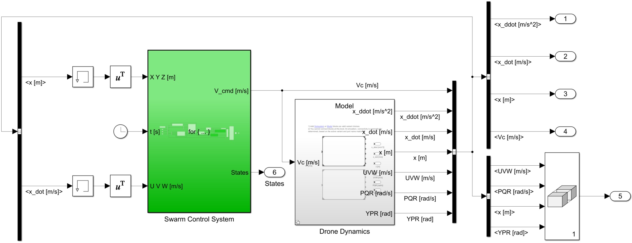
Figure 1.
Top-level block diagram of the swarm simulator
Two drone models were prepared. One is based purely on kinematics and simulates the three degrees of freedom (3DOF) movement of the point mass. This model, due to its fast computational time, can be used for a quick evaluation of the feasibility of the prepared mission plan. In this model, the commanded drone velocity, calculated for each of the drones by the swarm control algorithm, is directly equal to the drone’s actual velocity. The position is calculated by integrating this velocity.
The second model utilizes the full 6DOF rigid body movement. It includes a four-channel autopilot with control mixer, propellers model, and aerodynamic drag as well as atmosphere model including wind with constant speed and direction. This model can be used to accurately evaluate drones’ performance during mission execution.
The swarm control algorithm enables to flying of a swarm comprised of two types of drones: Leaders and Followers. There can be many Leaders flying simultaneously and each one of them can have multiple Followers arranged in a formation around them. The Leader drone is responsible mainly for tracking the specified trajectory given in the form of waypoints. The Follower’s mission is to simply follow the Leader, sticking to its predefined formation. Additionally, a formation reconfiguration possibility is implemented which allows for swapping the Followers between formation and base, e.g. after a low battery condition is detected. Drone’s 6DOF dynamics and swarm control algorithm are described in detail in the following sections.
3. Drone’s Dynamics
3.1. Coordinate systems
A set of coordinate systems was introduced to describe the quadrotor motion (Figure 2). The origin of the body-fixed frame Obxbybzb was attached to the quadrotor center of mass, Obxb axis is pointed forward, Obyb to the right, and Obzb down. North-East-Down (NED) coordinate system Onxnynzn was used to define the position of the drone in space. Additionally, gravity frame Ogxgygzg was used to obtain the loads from the gravity force.
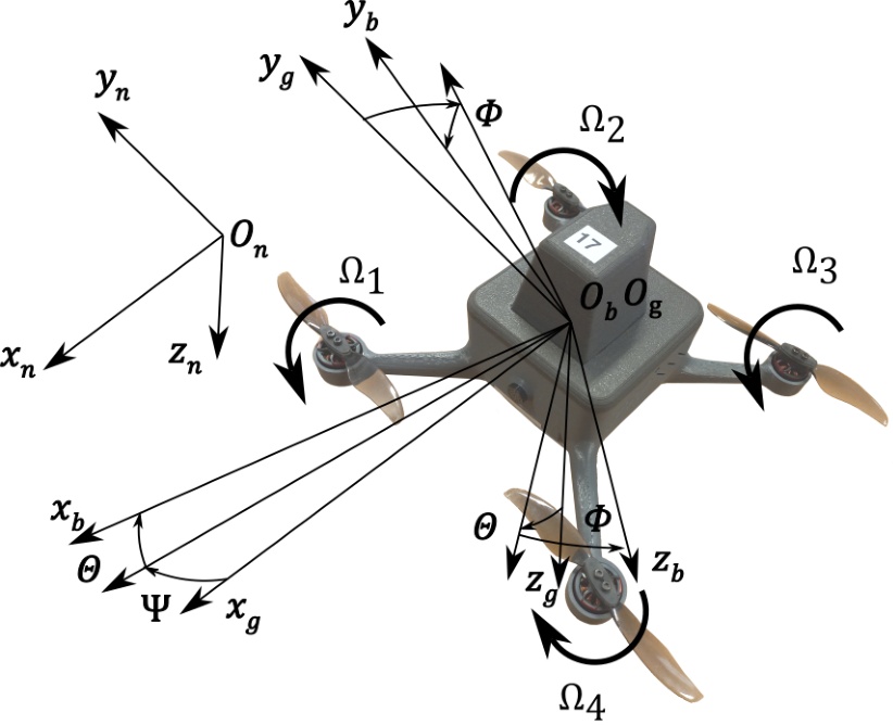
Figure 2.
Coordinate systems used in the simulation
3.2. Drones description
Both Leader’s (Figure 3) and Follower’s (Figure 4) are quadrotors in X-configuration propelled by brushless direct-current (BLDC) motors, although they differ in size. Leaders are bigger because a quite sophisticated autopilot was installed on the board to ensure appropriate computational resources. The directions of the propeller rotations are presented in Figure 2. Rotors 1 and 3 rotate counterclockwise (when looking from the top), and rotors 2 and 4 rotate clockwise.
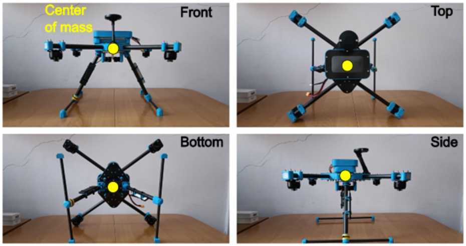
Figure 3.
Leader (with propellers removed)
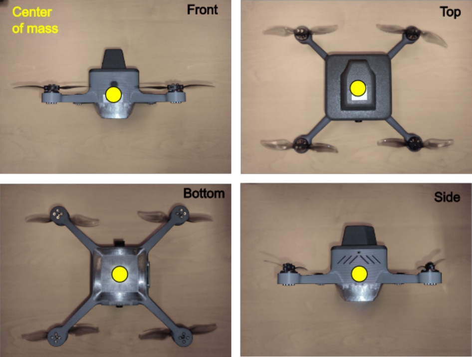
Figure 4.
Follower
The basic data of the Leaders are presented in Table 1 and Followers in Table 2, respectively.
Table 1.
Leaders’ parameters
| Parameter | Value |
|---|---|
| Mass [kg] | 2.182 |
| Moment of inertia Ixx [kg m2] | 0.055744 |
| Moment of inertia Iyy [kg m2] | 0.058427 |
| Moment of inertia Izz [kg m2] | 0.068685 |
| 1-st rotor location r1 [m] | [0.195, 0.135, 0]] |
| 2-nd rotor location r2 [m] | [-0.195, 0.135, 0] |
| 3-rd rotor location r3 [m] | [-0.195, -0.135, 0] |
| 4-th rotor location r4 [m] | [0.195, -0.135, 0] |
| Propeller diameter [m] | 0.3048 |
Table 2.
Followers’ parameters
| Parameter | Value |
|---|---|
| Mass [kg] | 0.274 |
| Moment of inertia Ixx [kg m2] | 0.000466 |
| Moment of inertia Iyy [kg m2] | 0.000476 |
| Moment of inertia Izz [kg m2] | 0.002024 |
| 1-st rotor location r1 [m] | [0.0775, 0.0775, 0] |
| 2-nd rotor location r2 [m] | [-0.0775, 0.0775, 0] |
| 3-rd rotor location r3 [m] | [-0.0775, -0.0775, 0] |
| 4-th rotor location r4 [m] | [0.0775, -0.0775, 0] |
| Propeller diameter [m] | 0.1016 |
Model parameters were obtained experimentally. Moments of inertia of the drones were measured using trifilar pendulum. The characteristics of the propellers were collected by static tests.
The maneuverability of the drones was limited programmatically in the autopilot settings. For the Leader, the roll and pitch angles fell into the range of ±30°. Ascent speed was 3 m/s, descent 3.4 m/s. For the Follower the roll and pitch angles are limited to ±35°, ascent/descent speed is ±3 m/s.
3.3. Drones simulation
The realistic dynamic model is crucial for understanding the swarming drone behavior. It was assumed that the sensors could perfectly measure the actual drone flight parameters. Also, the modeling of drone communication was omitted to simplify the analysis.
The equations of motion of the quadrotor are:
where m is drone mass, U, V, W are linear velocities, P, Q, R are angular rates, Xb, Yb, Zb are forces in body-fixed frame Obxbybzb. For rotational dynamics: where Lb, Mb, Nb are torques expressed in body-fixed axes. The net forces and moments were calculated as a sum of gravity, propulsion, and aerodynamic loads. The gravity forces are:Since the origin Ob of the body-fixed frame coincides with the center of mass, then the resulting torque from gravity is zero. Thrust force and torque generated by propellers were calculated as [28]:
where ρ is the air density, Sp is the rotor area, Rp is the propeller radius, Ωj is the angular rate of the j-th propeller, kf is the thrust coefficient, and km is the torque coefficient.Motor dynamics was modeled as a first-order system. The maximum possible angular rate of the propellers was limited using saturation.
The autopilot structure consists of four control channels (roll, pitch, yaw, and altitude). Proportional-integral-derivative (PID) controllers (with anti-windup protection) were used in each control channel. The PID controllers’ settings were tuned manually in flight tests of the actual objects and then used in the model.
A detailed description of the mathematical model and the controller structure can be found in [29].
The implementation of the drone’s dynamics is presented in Figure 5.
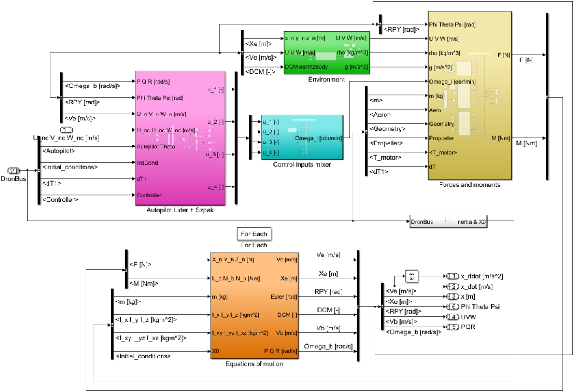
Figure 5.
Drone’s dynamic model developed in Simulink
The drone dynamic was implemented using ”For Each Subsystem” block. In that way, it was possible to realize the parallel simulations of multiple drones. Aerodynamic characteristics were tabulated as functions of angles of attack and sideslip.
Finally, the 6DOF drone dynamic model was optimized to achieve high computational efficiency. A built-in Simulink option called ”Accelerator mode” was used to reduce the time of numerical simulations. All unnecessary blocks were removed because they can significantly affect the simulation efficiency. This issue is crucial for the overall performance of the swarm simulator.
Next, the developed simulation module was validated using data from real experiments in outdoor conditions. A series of flight tests of the individual drones took place to obtain the data logs and identify the coefficients of the model. Two kinds of data logs were available. The data were logged on the onboard memory card and additionally sent by the telemetry to the ground control station. These files were analyzed using Mission Planner software and the UAV Log Viewer online service. Next, the gathered data were used to validate the developed models of Leader and Follower. Details about the model validation methodology can be found in [30].
4. Swarm Control Algorithm
The swarm control algorithm is divided into two parts – one for controlling the Leaders’ movement and the other for controlling the Followers’ movement. The swarm is divided into formations, usually based on a circle, consisting of one Leader and several Followers. The control algorithms’ outputs are commanded velocities, which are calculated for each drone as a weighted sum of several components depending on a few simple rules presented in Table 3 and Table 4 (see also Figure 6). The weights used to calculate the output velocity depend on the drone’s state and are tuned manually based on the simulation results. This velocity is then inputted to the drone’s autopilot or directly integrated when using the kinematic model.
Table 3.
Leaders’ control rules
| Rule | Description |
|---|---|
| Alignment | It ensures that the Leaders fly at an average velocity of all Leaders. |
| Cohesion | It ensures that the Leaders fly in a flock. |
| Separation | It ensures that the Leaders do not collide with each other. |
| Avoidance | It ensures that the Leaders do not collide with known, static obstacles. |
| Targeting | It ensures that the Leaders fly through their designated waypoints. |
Table 4.
Followers’ control rules
| Rule | Description |
|---|---|
| Alignment | It ensures that the Followers fly with the velocity of their Leader. |
| Cohesion | It ensures that the Followers tend to move to their Leader’s position. |
| Separation | It ensures that the Followers do not collide with each other within their formation. |
| Avoidance | It ensures that the Followers do not collide with known, static obstacles. |
| Formation | It ensures that the Followers keep the designated distance from each other within their formation. |
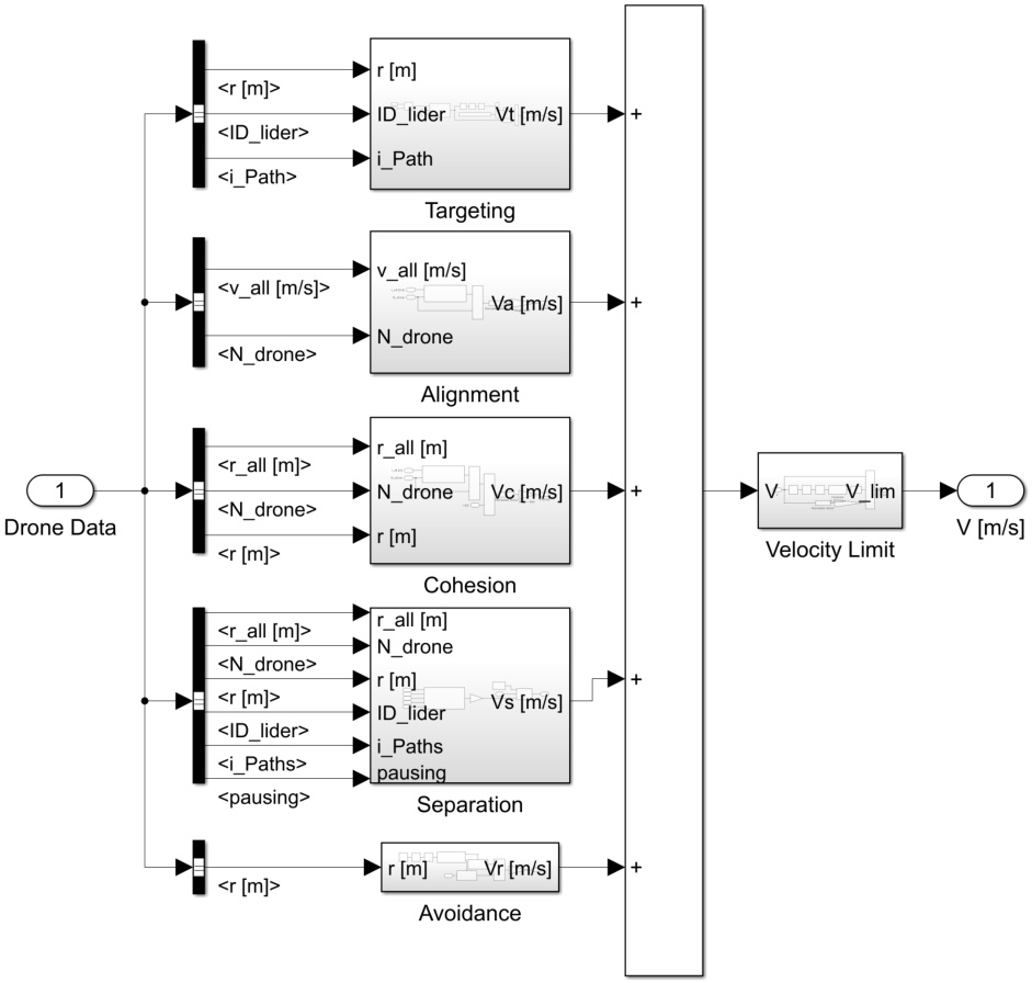
Figure 6.
Leaders’ control rules applied in Simulink
In the following sections, the details about the drones’ states and the transition between them, as well as the control rules for each of the states, will be provided, as it is a core of the developed algorithm that allows the efficient execution of the proposed mission.
4.1. Leaders’ states and transition conditions
Leaders can be assigned one of the six states, which are described in Table 5. The transition conditions between them are presented in the following paragraphs. Every Leader starts the mission in the Takeoff state.
Table 5.
Leaders’ states
| No. | Name | Description |
|---|---|---|
| 0 | Cruise | Main state in which the Leader flies through its designated waypoints. The Leader is allowed to wait in each of them for a specified amount of time, before flying to the next one. |
| 1 | Takeoff | State that is applied to the Leaders at the beginning of the mission. It indicates that the Leader is waiting in the base for the time when it is supposed to ascend or that it is ascending and waiting for the Followers to join it. |
| 2 | Landing | State in which the Leader, after reaching the last waypoint, is descending until it touches the ground. |
| 3 | Malfunction | State in which all communication with the Leader was lost and it is excluded from further calculations. |
| 4 | Standby | State in which the Leader awaits in the base for further instructions. |
| 6 | Return | State in which the Leader returns to the base. |
Transition from “1 – Takeoff” to “0 – Cruise”
While in the “Takeoff” state, the Leader awaits in the base for the ascend command for the predefined takeoff delay time, which allows the Leaders to start in a sequence. Then the Leader ascends to a set, intermediate altitude and awaits for the Followers to join and form a formation. After that, the Leader starts the flight through its designated waypoints.
Transition from “0 – Cruise” to “2 – Landing”
After the Leader reaches the last waypoint and the predefined waiting time for this waypoint passes, it transitions to the “Landing” state.
Transition from “2 – Landing” to “4 – Standby”
While in the “Landing” state, the Leader descends until it reaches a threshold altitude above the ground, where it waits for the Followers to achieve the Landing formation. Then the Leader starts descending further until touching the ground when it transitions to “Standby” state.
Other states
No transitions have been implemented between any other states yet.
4.2. Followers’ states and transition conditions
Followers can be assigned one of the seven states presented in Table 6. The transition conditions are presented in the following paragraphs. The Followers assigned to any of the formations at the beginning of the mission are starting in the “Takeoff” state. The Followers that will be replacing drones during reconfiguration are waiting in the base in the “Standby” state.
Table 6.
Followers’ states
| No. | Name | Description |
|---|---|---|
| 0 | Cruise | Main state in which the Follower flies in a formation and follows its Leader. |
| 1 | Takeoff | State that is applied to the Followers at the beginning of the mission. It indicates that the Follower is waiting in the base for the time of ascend or that it is ascending vertically before joining its Leader and forming a formation. |
| 2 | Landing | State in which the Follower is descending until it touches the ground. |
| 3 | Malfunction | State in which all communication with the Follower was lost and it is excluded from further calculations. |
| 4 | Standby | State in which the Follower awaits in the base for further instructions. |
| 5 | Flight to the Leader | State in which the Follower performs an independent flight to the Leader after takeoff from the base when one of the formations needs reconfiguration. |
| 6 | Return | State in which the Follower returns to the base after one of the formations needed reconfiguration. |
Transition from “1 – Takeoff” to “0 – Cruise”
The Follower that is assigned to one of the formations at the beginning of the mission awaits in the base for its Leader to start the ascend. Then, it ascends vertically to the intermediate altitude before transitioning to “Cruise” state.
Transition from “0 – Cruise” to “2 – Landing”
The Follower transitions from “Cruise” to “Landing” when its Leader transitions to “Landing” state, which happens when the Leader reaches it’s last waypoint.
Transition from “2 – Landing” to “4 – Standby”
During the landing phase, the Follower reaches a threshold altitude above ground while forming a landing formation. Then it descends until it touches the ground and transitions to “Standby” state.
Reconfiguration transitions – from “0 – Cruise” to: “2 – Landing”, “3 – Malfunction”, or “6 – Return”
There are three types of formation reconfiguration implemented that can happen during the mission. The condition that triggers these transitions in the simulation is the predefined time at which the event is supposed to happen (which can be changed to any other type of event, for example low battery condition during the real mission). In the case of the reconfiguration, the formation can be adjusted depending on the mission scenario. It can either reshape into a different circle-based figure, taking into account the decreased number of Followers, or stay the same by keeping one or more of its vertices empty. The Follower leaving the formation can either return to base, land directly below or become malfunctioned by transitioning to the appropriate state.
Transition from “6 – Return” to “2 – Landing”
If the Follower transitioned into the “Return” state it flew back to base. After reaching the base landing spot coordinates with appropriate accuracy, it transitions to “Landing” state.
Transition from “4 – Standby” to “1 – Takeoff”
When one of the Followers starts the reconfiguration and detaches from it’s formation, the other Follower that is assigned to fill a spot of a missing member of one of the formations gets the signal to ascend, it transitions to “Takeoff” to reach a designated altitude.
Transition from “1 – Takeoff” to “5 – Flight to the Leader”
After reaching the designated altitude during the ascend, the Follower transitions to “Flight to the Leader” state and flies towards the Leader.
Transition from “5 – Flight to the Leader” to “0 – Cruise”
After the Follower reaches the Leader, it transitions to “Cruise”, attaches to the formation, and begins its flight following the Leader.
Other states
There are no transitions implemented between any other states yet.
4.3. Leader’s trajectory control
The Leader’s control algorithm is comprised of a set of rules from Table 3 and differs depending on the state in which the Leader currently is. Before going into the autopilot is it caped at the predefined maximum allowable speed to prevent controller’s misbehavior, see also Figure 6. The control rules are straightforward due to the fact that they will need to be executed on small microcontrollers inside the drone, with very limited memory and computation capabilities.
Cruise state
In the Cruise state, which is a nominal state for a Leader, the control algorithm consists of five rules: Targeting, Alignment, Cohesion, Separation, and Avoidance. The resulting commanded velocity is a weighted sum of all five rules.
The Targeting rule’s purpose is to steer the drone into the direction of the next waypoint. The commanded velocity for this rule is calculated as:
where wT is the weight, rT is a waypoint position, and r is the position of the drone. When the drone is closer to the waypoint than the predefined threshold value, the target is switched to the next waypoint. The drone can also wait at the waypoint for a specified amount of time.The Alignment rule makes the drone fly with the average velocity of all of the Leaders in the average direction. The commanded velocity is calculated as:
where wA is the weight, vi is the velocity of the i-th Leader, and N is the number of Leaders.The Cohesion rule forces the drone to fly to the geometric center of all of the Leaders’ positions. The overall purpose of this rule is to keep the drones in a group or flock. The commanded velocity is given by:
where wC is the weighting factor, ri is the position of the i-th Leader, N is the number of Leaders, and r is the position of the drone.The Separation rule forces the drone to avoid collisions between any other Leaders. Also, due to the fact that every Leader is surrounded by the formation of Followers, this rule avoids the collisions between individual formations keeping the Leaders separated by a distance greater than the sum of their formation radii. Its commanded velocity is given as:
where wS is the weighting factor, which is adaptive based on the distance between drones, ri is the position of the i-th Leader, N is the number of Leaders, and r is the position of the drone. This rule has additional conditions. It is switched off whenever the drone is further away from any other Leaders than the specified threshold or if there is a sufficient difference in height at which two Leaders are flying.The last rule is the Avoidance. This rule prevents the Leader from colliding with stationary obstacles of a known position. The commanded velocity is calculated as:
where wR is the weighting coefficient, which is adaptive based on the distance between the drone and the obstacle, rPi is the position of the i-th obstacle, N is the number of obstacles, and r is the position of the drone.Takeoff state
In the Takeoff state, which is an initial state for a Leader, the control algorithm consists of two rules: Targeting and Separation. The resulting commanded velocity is a weighted sum of the rules. In this state, the Leader is waiting in a base for a Takeoff command and then ascending to the intermediate height to weight for the Followers to join and form a formation. The Separation condition is identical to the one described in the Cruise state paragraph.
The Targeting rule’s purpose is to ascend the drone to an intermediate height. The commanded velocity for this rule is calculated as:
where, wT is a weighting coefficient, hT is the intermediate height, and rz is the vertical component of the position of the drone.Landing state
In the Landing state, the control algorithm consists of only one rule: Targeting. In this state, the Leader is located at its last specified waypoint. It then descends to the intermediate altitude and waits for the Followers to achieve the landing formation and then descends further until reaching the ground.
The commanded velocity for the Targeting rule in this stat is calculated as the one described in the Takeoff paragraph for the first part of the maneuver and for the second part with the equation:
where, wT is the weight and r is the drone’s position.Return state
In this state, the Leader is flying back to the base. The control algorithm consists of three rules: Targeting, Separation, and Avoidance. All of the rules are almost identical to the ones described in the paragraph regarding the Cruise state. The only difference is in the Targeting rule, where the waypoint’s position is replaced by the base landing coordinates. The Leader is flying directly above the Landing place and then switches to the Landing state where it performs the Landing maneuver.
Other states
There are no algorithms implemented in “Malfunction” and “Standby” states.
4.4. Follower’s trajectory control
The control algorithm of a Follower is comprised of a set of rules from Table 4, very similar to the rules for a Leader, and differs depending on the state in which the Follower currently is. Before going into the autopilot it is also capped at the predefined maximum allowable speed to prevent the controller’s misbehavior.
Cruise state
In the Cruise state, which is a nominal state for a Follower, the control algorithm consists of five rules: Formation, Alignment, Cohesion, Separation, and Avoidance. The resulting commanded velocity is a weighted sum of all five rules.
The Formation rule is responsible for keeping all of the Followers of a particular Leader in a formation. It makes the followers keep the desired distances between them during the flight. The equation for the commanded velocity is given as:
where wF, kp, and kd are weighting factors, N is the number of Followers in the formation, ri, vi are the position and the velocity of every Follower in the formation, and r, v are the position and velocity of the current Follower. The M is given by: where Mx, My, Mz are the mutual distance matrices that hold the distances between each Follower in x, y, and z position coordinates that are calculated using the equations: where R is the radius of the formation and α is the angular position of the Follower in that formation given as: where θ is the formation angular offset.The Alignment rule makes the Follower fly with the velocity vector of its Leader. The commanded velocity is calculated as:
where wA is the weight, and vL is the velocity of the Leader.The Cohesion rule is forcing the Follower to fly to the position of the Leader. The overall purpose of this rule is to keep the formation around the Leader during the flight. The commanded velocity is given by:
where wC is the weight, rL is the position of the formation Leader, N is the number of Followers in the formation, and ri is the position of the i-th Follower.The Separation rule forces the drone to avoid collision with any other Followers inside the formation. Its commanded velocity is given by the equation analogous to the Leader’s rule. The Avoidance rule prevents the Follower from colliding with stationary obstacles of a known position. The commanded velocity is calculated in the same way as for the Leader.
Takeoff state
This state is separated between two types of Followers. The first type is the Follower which starts as a member of a formation. This type of Follower in this state is firstly waiting for the Takeoff of its Leader and then is ascending vertically for a few seconds before transitioning to the Cruise state. The second type of the Follower is a part of the reconfiguration procedure. This type obeys two rules in this state: Targeting and Separation. The latter one is almost the same as for the Cruise state, with the difference that the Follower is avoiding the collision between other Followers in the Reconfiguration condition.
The Targeting rule’s purpose is to make the Follower achieve the appropriate altitude at which it will be continuing the flight toward the Leader. The commanded velocity for this rule is calculated as:
where, wT is a weight, hT is the commanded altitude and rz is the vertical position of the drone.Landing state
This state is the same as the one described for the Leader.
Flight to the Leader state
This state is a part of the Reconfiguration process. In this state, the Follower is flying towards the Leader in order to join its formation. It obeys three rules: Targeting, Separation, and Avoidance. The Avoidance rule is the same as for the Leader, and the Separation is the same as in the Takeoff state for the Follower.
The Targeting’s rule purpose is to steer the drone in the direction of a Leader. The commanded velocity for this rule is calculated as:
where, wT is a weight, rL is a Leader position with the offset on the vertical position in order to avoid collisions with other flying formations, and r is the position of the Follower. When the drone is closer to the Leader than the predefined threshold it joins the formation and switches to the Cruise state.Return state
This state is a part of the Reconfiguration process. In this state, the Follower is flying towards the base. It obeys three rules: Targeting, Separation, and Avoidance. All of the rules are the same as for the Flight to the Leader state. In the Targeting rule the target is the base landing point. The Follower is flying at a different altitude than all of the formations and Followers in the Flight to the Leader state in order to avoid collisions.
The Targeting rule’s purpose is to steer the drone in the direction of a Leader. The commanded velocity for this rule is calculated as:
where, wT is a weight, rL is a Leader position with the offset on the vertical position in order to avoid collisions with other flying formations, and r is the position of the Follower. When the drone is closer to the Leader than the predefined threshold it joins the formation and switches to the Cruise state.Other states
There are no algorithms implemented in “Malfunction” and “Standby” states.
5. Mission Description
The purpose of the prepared swarm control algorithm is to cover a specified area with a grid of drones for the purpose of establishing a WiFi network in emergency situations. In order to take into account the battery life of the drones the grid is filled using a “snake” pattern, as shown in Figure 7.
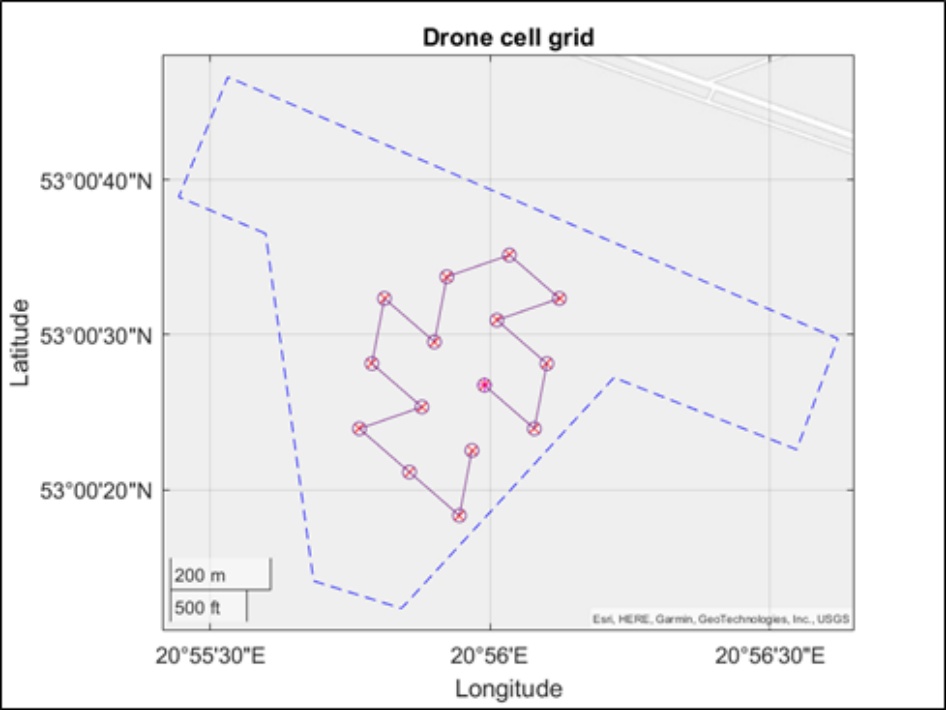
Figure 7.
The snake pattern for a grid coverage
There are fifteen cells in the prepared grid which will need fifteen Leaders to fully cover it. Each of the Leaders has six Followers in the formation which gives 105 drones in total. Each of the formations will start sequentially from the same place marked with a red dot in Figure 7, and will follow the pattern until it reaches the last way-point shown. In all of the way-points, the Leaders will wait for a specified amount of time, dependent on the battery life and the overall required length of the mission. To avoid collisions between the formations, especially in the turns, and to preserve the necessary distances between the drones for communication and WiFi coverage purposes, every other formation will be flying at a different altitude, even-numbered formations higher and odd-numbered formations lower than the way-points’ defined height. After reaching the last way-point shown (second to last of the mission), the formations will proceed to the landing zone obeying the rules of the formation landing sequence. In the next section, the detailed simulation results will be presented.
In this particular scenario, each formation starts with a delay of 90 seconds with respect to the previous one and waits at each of the way-points for 25 seconds. Every formation has a radius of 50 meters during the flight, which shrinks to 5 meters during the landing phase. The distance between every way-point is equal to 132 meters and between the second to last and the last to 561 meters. The way-points are located at the height of 120 meters, even formations are flying 5 meters above them, and the odd ones 5 meters below, to avoid collisions. The formations are moving at a speed of 3 meters per second.
6. Simulation Results
The swarm control algorithm was run for the mission described in the previous section. The computations were performed on the standard desktop computer (equipped with an Intel Core i7 CPU and 32 GB RAM). The formations were starting sequentially from the same starting position, as shown in Figure 8. The Leaders are marked purple, and the Followers are light blue, the way-points are shown as green circles. The trajectory is made of 15 way-points with one additional, different for every Leader, in the top left corner reserved for landing. All of the formations follow the same path, only the landing points are unique for each of the formations. Additionally, at the top of the graph, the actual time (in seconds) of the mission is presented.
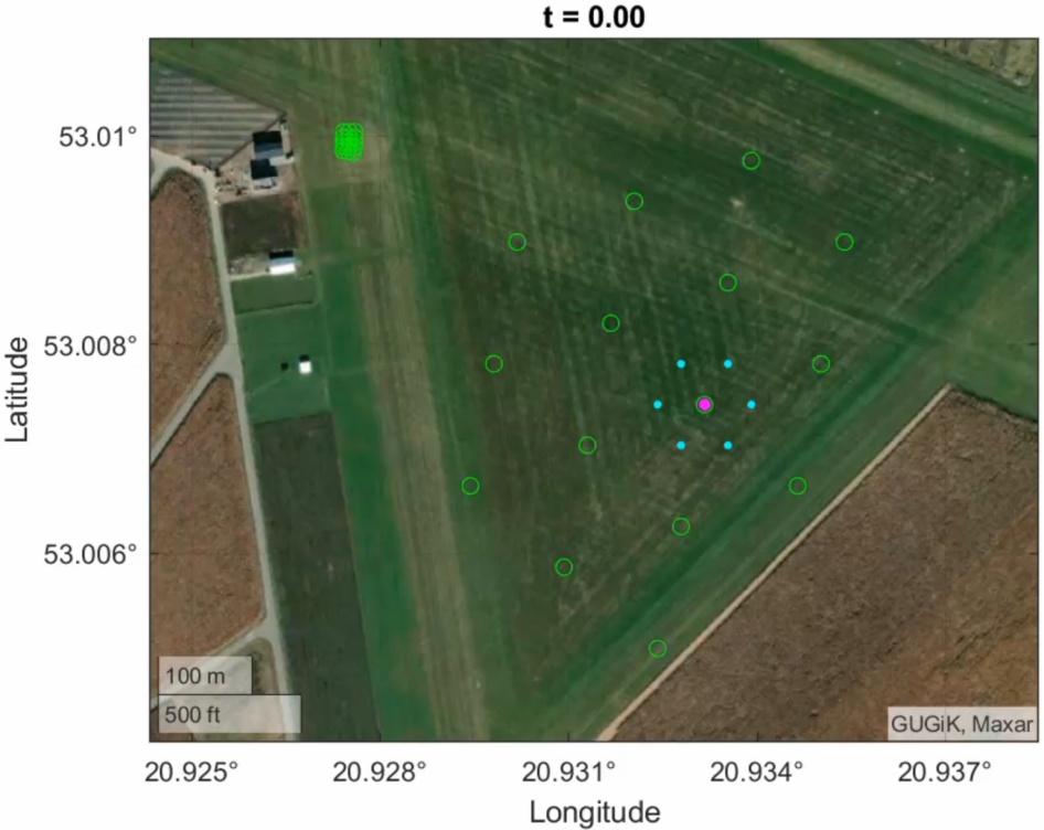
Figure 8.
Beginning of the mission
An important aspect of the algorithm is the precise tuning of all of the algorithm’s parameters. To cover up the whole grid at the same time, it is necessary to specify the start time delay for all of the Leaders and their way-points wait time. As can be seen in Figure 9 the drones are starting to fill out the space, keeping the necessary distances required for effective communication and collision avoidance. When all of the drones are in the air, see in Figure 10, all of the way-points are fully covered.
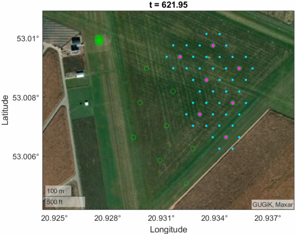
Figure 9.
Drones filling up the grid
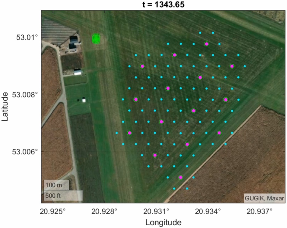
Figure 10.
All of the drones are in the air
After completing the main part of the trajectory, the formations proceed to the last waypoint, where they perform the landing procedure, as shown in Figure 11. The formations are reducing their radii, and the whole group is landing in the set coordinates. The whole mission took 50 minutes to complete. Because of all of the control rules and the spread of altitudes between the respective formations, there are no collisions during the flight.
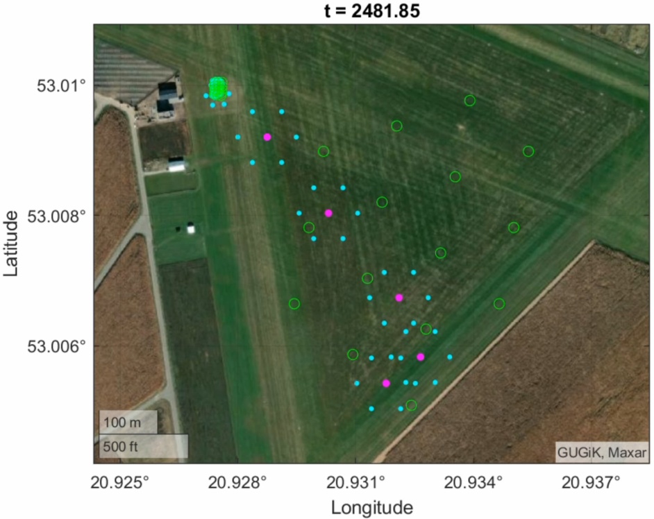
Figure 11.
Return to the landing zone
7. Conclusions
In the presented study, a full 6DOF drone swarm simulator created in MATLAB/Simulink was presented and described. An efficient swarm control algorithm was developed that allows it to cover a specified area with a grid of drones. The simulator allows taking into account environmental conditions like wind, terrain heights, and drone battery supply for the purpose of establishing a WiFi network in emergency situations. Several contributions in the field of an autonomous swarm of drones might be mentioned.
The results of the prepared simulation show that the area can be effectively and fully covered by the drone formations, without in-flight collisions, and keeping the necessary distances between the drones. In the considered scenario, the Leaders moved along a predefined flight path. It was found that regular hexagons are the most suitable formation shapes to cover the whole region.
The developed simulator has a modular structure and is highly customizable. The data of other quadrotors can be easily implemented. Moreover, the developed software is scalable and allows for performing simulations for a large number of drones. The software user can define various simulation scenarios. Calculations can be easily performed on the standard desktop computer without the need to use sophisticated computational resources (like workstations or clusters). This is a significant advantage when compared to existing simulators (for example, Gazebo).
However, one of the most challenging issues is to set the appropriate parameters of the proposed control algorithm. In the presented study, these parameters were tuned manually by trial and error method, which is quite a time-consuming task. When some significant changes in the system configuration are introduced, then these weights must be tuned again to meet the desired performance. In the future, automatic tuning methods should be used to make this process more effective.
It is possible to achieve complicated swarm behavior using a set of relatively simple mathematical rules. This feature is important from a practical point of view because of the limited onboard computational resources. Simple algorithms can be easily implemented in the autopilot software.
The mission was completed in about 50 minutes. In the real system, the drone must be equipped with an onboard battery with the appropriate capacity to realize the whole mission. This is a significant problem when small drones are used as Followers because they cannot carry heavy batteries and must be replaced by drones with fully charged batteries during the mission, complicating the task. Future plans include modeling the drone battery usage and using that information to drive the reconfiguration process during the simulation.
The developed simulator can be practically used for flight test planning purposes. In the near future, the drones’ dynamic model and proposed swarm control algorithm will be validated using the data obtained experimentally during flight tests in outdoor conditions. The influence of drone failure on the performance of the whole formation should be studied in detail. The effects of communication delays and signal losses must also be investigated.
ACKNOWLEDGEMENTS
This work was supported by the National Centre of Research and Development under POIR programme under research project agreement POIR.01.01.01-00-0040/22