

1. Introduction
Coverage Path Planning (CPP) is a fundamental problem in mobile robotics. CPP aims to compute a route that passes over all points in a given area or volume while avoiding obstacles [1]. This task is integral to many robotic applications such as agricultural field operations, floor cleaning, and automated lawn mowing [2]. The key objective in CPP is to minimize the total traversal time and energy of the robot while ensuring full coverage of the target area. Because robots often have differential-drive or car-like dynamics, smooth paths with few sharp turns are preferred to reduce wear and energy use.
A common strategy is to decompose the environment into simpler subregions before path planning. For example, classical methods partition free space into cells (trapezoids or boustrophedon cells) or use grid-based spanning-tree coverage. In each subregion, a systematic sweep pattern (such as boustrophedon or spiral) is used [3,4,5]. This approach has been summarized as three steps [6]: (1) divide the environment into smaller regions (cells) for coverage, (2) compute a coverage path for each region and an order to visit them, and (3) smooth the overall path. Our work follows this outline but enforces oriented rectangular regions. Rectangular segmentation has distinct advantages: as shown in prior work, an axis-aligned back-and-forth sweep will exhaustively cover a rectangular area without any redundant overlap [3]. This yields coverage paths that consist of long straight segments and only the necessary turns, improving smoothness and trackability.
This paper focuses on CPP in real-world operational maps. We assume a known occupancy grid of the environment, such as an office or warehouse floor plan. We emphasize efficiency in practical settings: the robot must cover all accessible areas while reducing idle motion.
The research described in this paper originates from the practical requirements of an industrial cleaning robot, which aimed to find the best coverage path of any real-life environment. A typical characteristic of maps recorded by robots in real-life conditions is the presence of noise, which prevents decomposing such maps into regular geometric primitives. Assumption of regular shapes is however, a bottom line for most State-of-the-art algorithms. Throughout the research, we found that these algorithms solve very well the CPP problem on artificially created maps composed of regular polygons. When however applied to real-life maps, these algorithms generate unlikely paths as shown in Figure 5. To address this practical challenge we propose to adapt a decomposition strategy similar to the one a human operator would follow and divide the map into segments approximated by rectangles. This allows our algorithm to create paths that avoid unnecessary crossings of already cleaned floor.
The key novelty of this work is the iterative fitting process: a gradient-based optimization loop in which rectangle parameters (position, size, and orientation) are treated as continuous variables and refined via a differentiable rectangle function. Unlike classical decomposition methods that rely on exact geometric primitives, our differentiable formulation provides non-zero gradients across the image domain, enabling smooth, stable convergence even on noisy occupancy grids. Crucially, the gradient descent steps are interleaved with structural operations—merging overlapping rectangles, deleting insignificant ones, and splitting rectangles that span disconnected regions—which reshape the decomposition topology and allow the optimizer to escape local minima. This combination of continuous parameter optimization with discrete structural adaptation is what enables robust segmentation of real-world maps.
In summary, we introduce a gradient-based adaptive algorithm that partitions a given map into rectangular zones and generates the corresponding coverage path. The main contributions are:
A differentiable rectangle function that enables gradient-based optimization of rectangle parameters on occupancy grids, providing non-zero gradients where classical binary representations would yield zero or undefined derivatives.
An iterative fitting process that combines continuous gradient descent with discrete structural operations (merge, delete, split), enabling robust rectangular segmentation of noisy, real-world maps where conventional decomposition methods fail.
An empirical evaluation on large-scale real-world maps demonstrating that the proposed method yields smoother coverage paths with significantly reduced curvature and execution time compared to baseline methods.
2. Related Work
Complete Coverage Path Planning has been extensively studied in the robotics literature. Multiple reviews have been published that classify and analyze existing approaches. [7] provides algorithmic frameworks organizing work into heuristic and randomized methods, as well as provably complete approaches based on cellular decompositions, including approximate, semi-approximate, and exact decompositions. [1] surveys how different algorithms decompose and represent environments to generate complete coverage paths, reviewing exact cellular decompositions such as trapezoidal and boustrophedon methods, Morse-based approaches that handle complex obstacle geometries, and grid-based methods using wavefronts, spanning trees, or neural networks. [6] focuses on the main methodological components of environment decomposition, coverage execution, backtracking sequence planning, and path smoothing, surveying decomposition strategies such as cell-based, grid-based, sampling-based, and spanning-tree approaches.
More recent comprehensive reviews include [8], which presents a comparative performance analysis of several coverage path planning algorithms, and [9], which explores various CPP approaches for Unmanned Aerial Vehicles, dividing methods into three main groups: no decomposition (simple patterns), exact cellular decomposition, and approximate cellular decomposition. [10] reviews classical and heuristic algorithms with emphasis on optimization characteristics, while [11] focuses specifically on complete coverage path planning for precision agriculture with emphasis on exact cellular decomposition methods. Finally, [12] provides a comprehensive survey for static and dynamic environments, classifying methods into grid-based, graph-based, sampling-based, and optimization-driven approaches.
Based on these comprehensive reviews, complete coverage path planning can be understood as a three-step process: (1) segmentation or decomposition of the environment into manageable regions, (2) coverage path planning within each region, and (3) sequence optimization to determine the optimal order to visit regions. The decomposition method fundamentally influences the quality of generated coverage paths.
2.1. Cell Grid-Based Methods
Grid-based methods divide the environment into a regular grid of cells and generate a coverage path that visits all cells. These methods represent an approximate cellular decomposition approach, where no sophisticated decomposition structure is imposed beyond the regular grid structure itself.
Spanning tree coverage methods.
The spanning tree coverage approach was introduced by [13], which decomposes the free space into mega cells and constructs a spanning tree that traverses all cells; the robot covers the entire area by following the tree’s boundaries and visits four smaller cells within each mega cell. This graph-based representation can guarantee complete coverage in structured environments with few obstacles, but it generates a single, continuous path without decomposing the environment into operational zones and can be computationally expensive for large or highly complex maps. Recent extensions by [14] and [15] improve efficiency through cell reduction, yet still produce monolithic coverage paths.
Neural network-based coverage path planning.
[16] proposed a neural dynamics-based approach for complete grid coverage using neural networks, leveraging activation patterns to guide navigation across grid-structured environments. While this provides distributed decision-making and can handle complex grid patterns, it is only effective on simple maps and requires a very dense grid, leading to prohibitive memory and computational demands for large industrial environments such as warehouses.
2.2. Exact Cellular Decomposition Methods
Exact cellular decomposition methods break the free space into simple, non-overlapping regions called cells. These cells are typically defined based on the geometric and topological properties of the environment. Once decomposition is complete, a simple motion pattern (such as back-and-forth motions) is applied within each cell to ensure complete coverage.
Boustrophedon decomposition.
The boustrophedon cellular decomposition method was introduced by [3]. It is based on trapezoidal decomposition, but improves efficiency by identifying critical points that separate distinct connectivity changes and thus produces fewer cells. The method divides free space into trapezoid-shaped cells via sweep lines from polygonal obstacle vertices and then applies simple back-and-forth motions within each cell. This yields exact coverage guarantees with an easily traversable cell structure, while still relying on polygonal, well-structured environments.
Morse-based cellular decomposition.
[17] generalized decomposition using critical points of Morse functions, enabling decomposition based on distance-function properties rather than polygonal obstacle definitions. This can handle non-polygonal obstacles and complex geometries with theoretical coverage guarantees, but extensions such as [18] remain targeted at relatively structured environments with clear boundaries and do not directly scale to large, unstructured maps which can include multiple rooms, narrow corridors, and irregularly shaped spaces.
2.3. Bio-Inspired and Optimization-Based Methods
Bio-inspired and metaheuristic algorithms have been increasingly applied to coverage path planning, either for directly generating coverage paths or for optimizing the sequence and routing of pre-computed coverage sub-regions.
Genetic algorithm-based approaches.
Genetic algorithms (GA) simulate natural evolution to explore the solution space. [19] applied GA to coverage path planning by encoding paths as chromosomes and using selection, crossover, and mutation, with later applications in agricultural coverage [20] and irregular regions [21]. These methods can optimize multiple criteria such as path length and coverage quality without strict geometric assumptions, but they are computationally expensive at scale and do not inherently decompose the workspace, often producing paths that jump between distant regions rather than supporting zone-by-zone industrial operations.
Ant colony optimization.
Ant Colony Optimization (ACO) uses swarm intelligence, where virtual ants deposit pheromone trails that guide subsequent search toward promising solutions. [22] developed a fast-spanning ACO method for mobile robot coverage, and [23] combined simulated annealing with ACO for interior cleaning applications. ACO can find near-optimal solutions and handle constraints, but it explores a large search space, tends to converge slowly in large industrial maps, and does not impose a decomposition structure, limiting its ability to produce meaningful operational zones.
2.4. Recent Advances and Specialized Applications
Recent work in coverage path planning has addressed specialized application domains and attempted to tackle limitations of earlier approaches. [24] proposed a calculation-based shortest path search algorithm (CbSPSA) for marine survey applications, partitioning irregular polygon areas into convex sub-regions for efficient coverage. [25] developed an improved spanning tree coverage method with optimized backtracking for large-scale unstructured social environments (cleaning tasks). [26] integrated Building Information Modeling (BIM) with coverage path planning for indoor robot applications, incorporating semantic enrichment of maps to improve coverage efficiency.
For agricultural applications, [27] proposed hybrid path planning combining nested and spiral methods for harvesting operations in convex polygonal fields. [28] developed a Voronoi-based decomposition framework for large outdoor sweeping operations, demonstrating that Voronoi decomposition outperforms grid-based decomposition. [29] addressed coverage planning in semi-structured outdoor environments by combining map preprocessing with coverage path planning to maximize coverage efficiency. Finally, [30] introduced Fields2Benchmark, a modular benchmark for standardizing evaluation of agricultural coverage path planning, decomposing the problem into field decomposition, headland generation, swath generation, route planning, and path planning stages.
While these methods address specific application domains and achieve improvements in efficiency, they typically still rely on either: (1) decomposition methods that assume structured or convex environments, (2) optimization techniques that do not inherently segment the workspace into manageable operational zones, or (3) specialized approaches tailored to particular problem structures that lack generalizability to arbitrary environments.
2.5. Analysis and Motivation
Existing CPP methods either generate monolithic coverage paths on grids, assume polygonal structure for exact decomposition, or optimize paths without enforcing meaningful segmentation, which makes them ill-suited to large, unstructured maps that require zone-by-zone operation. Most existing methods either assume idealized map conditions or require extensive preprocessing to be effective, and many fail to adapt efficiently to the irregular, noisy maps encountered in real-world warehouse environments. There is thus a clear gap in segmentation methods that can scale to industrial-sized environments while producing operationally practical, separable coverage zones. We therefore introduce our method to decompose complex layouts into efficient rectangular zones that can be covered independently. By leveraging geometric regularities and gradient information to simplify map structure while adapting to obstacle distribution, our approach enables robust, efficient, modular, and scalable path planning in large-scale cleaning tasks.
3. Problem Description
We address the problem of generating a complete coverage path over a known 2D occupancy grid M of size W × H with resolution r (pixels per meter). Free cells (value 1) represent traversable areas, and occupied cells (value 0) represent obstacles. The objective is to compute a route that covers all accessible areas with minimal path cost, defined in terms of length, curvature, and execution time.
Formally, given the grid map M and resolution r, we seek a partition of free space into the smallest and least numerous set of rectangular areas {R1, … , Rn}. Each Ri is an axis-aligned rectangle specified by its center, width, height, and orientation. A coverage path is then planned so that each zone is fully swept.
To evaluate path quality, we use the following metrics:
Length per square meter (AL):
where Lroute is the total path length (m), and Ncovered is the total area (m2) effectively covered by the robot. This metric reflects the efficiency of movement—lower values indicate less distance traveled per unit area cleaned.Coverage ratio (C):
where Nfree is the total free area in the map. This metric quantifies completeness of coverage—ideally close to 1, indicating minimal missed regions.Curvature per square meter (κ):
where Δθ are turn angles along the path. High curvature implies frequent direction changes, which may slow execution or introduce mechanical wear, especially in large or cluttered environments.Time per square meter (T):
where Ttotal includes estimated execution time, incorporating robot kinematics such as maximum velocity, acceleration limits, and time spent stopping and turning. This reflects real-world performance, prioritizing motion plans that are not just short but also smooth and feasible.
3.1. Cleaning Time Estimation
The total cleaning time is estimated by modeling the robot’s motion constraints, including maximum linear and angular velocities ( ) and accelerations ( ).
The path is segmented into linear and turning segments. For each linear segment, the time is computed by considering acceleration and deceleration phases to and from cruising speed, ensuring the robot respects acceleration limits. For turns, the time is estimated based on the angle turned, accounting for maximum angular velocity and acceleration, assuming the robot stops to rotate in place.
Formally, the total time is the sum of:
where each component is calculated as:Tlinear : Time to traverse straight paths with acceleration/deceleration phases
Tturn : Time to perform stationary rotations given angle and angular acceleration constraints
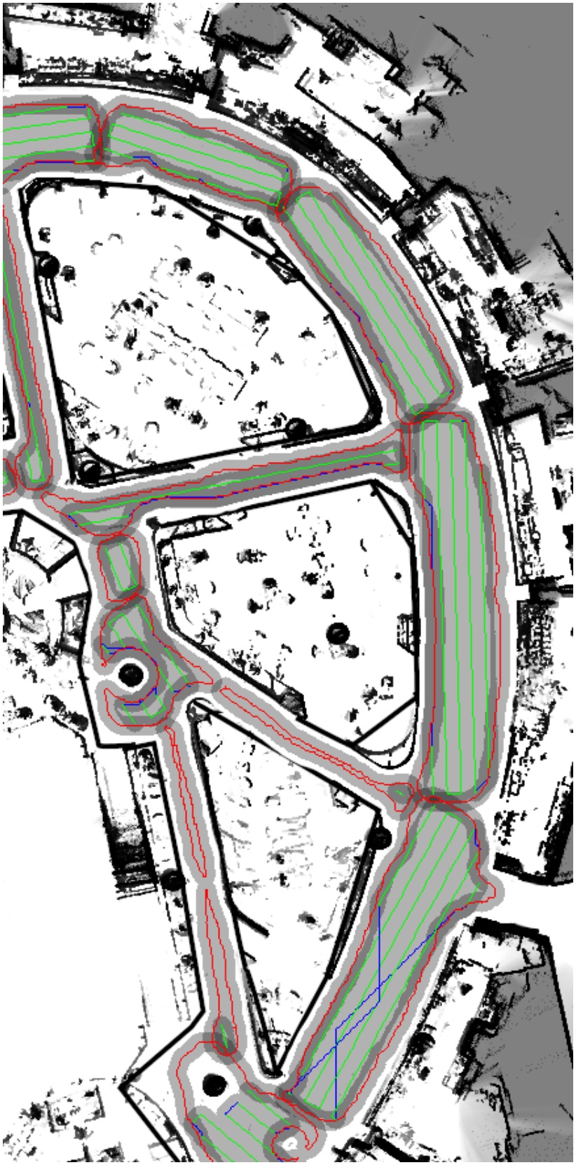
Figure 1.
Coverage paths generated by the Gradient-Based Rectangular Segmentation method. Red, green, and blue lines represent wall-following, boustrophedon, and A* paths, respectively. Grayscale intensity indicates coverage frequency, with darker regions representing areas covered multiple times
This approach realistically estimates the robot’s cleaning time considering kinematic constraints and motion phases.
4. Methodology
Our CPP pipeline has three main stages: (1) segment the map into rectangular zones, (2) generate a local coverage path in each zone, and (3) sequence the zones into a global path. The algorithm is implemented in Python and takes a binary occupancy grid as input.
The goal of the segmentation step is to take an input map and generate the smallest and least numerous set of rectangles that cover the entire open space.
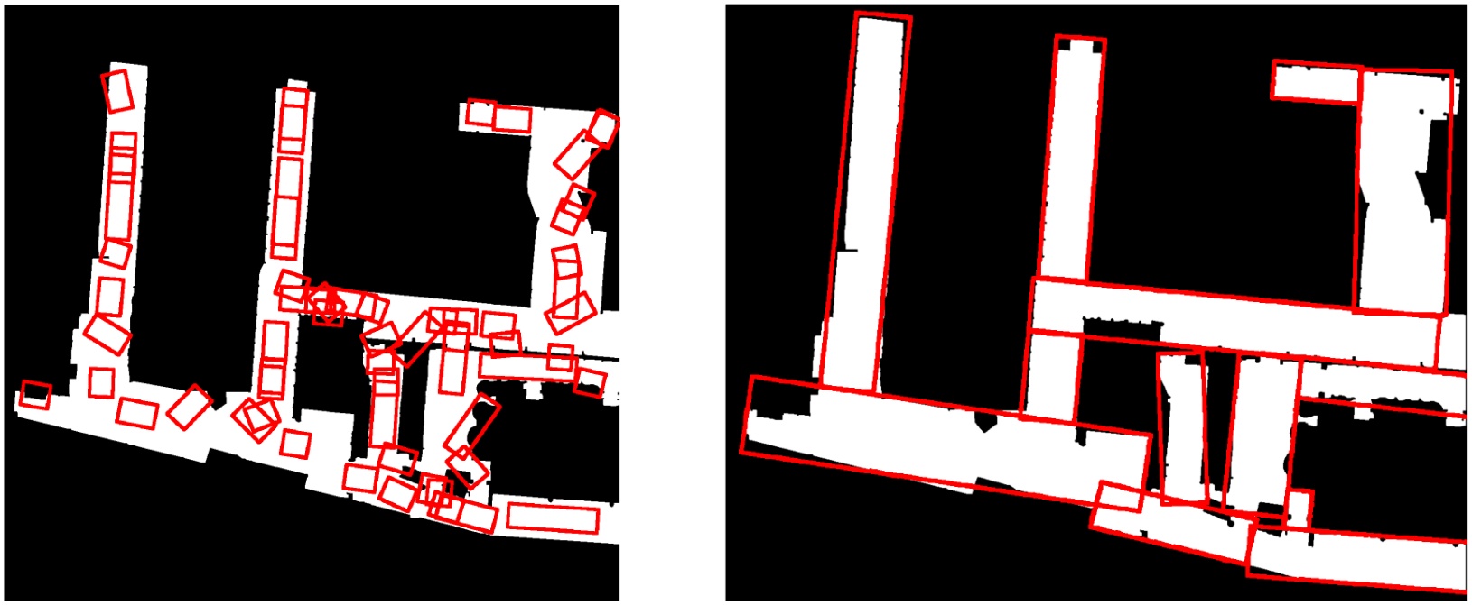
Figure 2.
Comparison of initial (left) and regressed (right) rectangles
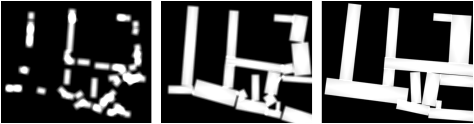
Figure 3.
Progression of rectangle representation during optimization steps after 3 steps (left), 30 steps (middle), 300 steps (right)
To achieve this, we employ an optimization approach based on gradient descent, which minimizes the error between the real map and a model of the map represented as the sum of several rectangular regions. Below, we outline the key components of our segmentation process.
4.1. Initial Rectangle Generation
The initial set of rectangles should approximately cover the area of interest, providing a starting point for the optimization process. For this task, we utilize a Voronoi decomposition of the map to divide it into regions that approximate the open spaces. We then apply the probabilistic Hough transform to identify the directions and centers of most rooms and corridors. Using these center points, we define initial rectangles by assigning each position and length of the corresponding line, with a predefined width.
4.2. Rectangle Fitting via Gradient Descent
Once the initial set of rectangles is defined, we apply a gradient descent algorithm to refine the fit of these rectangles to the open spaces in the map. The goal is to adjust the position and dimensions of each rectangle to minimize the difference between the actual map and the sum of the rectangles.
The objective function to be minimized is defined as:
where:R is the matrix of rectangle parameters, with each row representing a different rectangle.
r(Rj) is the rectangle function, which takes the parameters of a rectangle Rj (position x, y, width w, height h, and rotation angle r) and returns an image of the rectangle. This parameterization was specifically chosen to ensure parameter space continuity during Gradient Descent. By defining the rectangle via its center (x, y) and a continuous rotation angle θ, we avoid the ‘jump’ discontinuities that occur when using corner-based coordinates. This ensures that infinitesimal updates to the parameters result in smooth, predictable transformations of the rectangle geometry.
M is the input map.
J(R) is a regularization term that penalizes overly small rectangles, encouraging the replacement of smaller rectangles with larger ones. Here w(R) and h(R) refers to width and height of the given rectangle respectively
The main objective is to ensure that the sum of the rectangle images closely matches the input map, while minimizing the number of unnecessary or redundant rectangles.
4.3. Coverage Enhancement through Weighted Objective Function
While the basic objective function (Eq. 6) treats all pixel-level errors equally, in practice uncovered free space is more detrimental to cleaning performance than minor overlaps or overestimation. To address this asymmetry, we introduce a per-pixel weighting scheme that amplifies the penalty for pixels where the map indicates free space but the current rectangle configuration fails to cover it.
Let denote the sum of all rectangle functions and ei,j = Si,j − Mi,j the per-pixel residual. We define a weighting function w(ei,j) that assigns different importance to each pixel based on the sign of its residual:
where α > 1 is a weighting parameter that controls how strongly the optimizer prioritizes covering free space over reducing other errors. The modified objective function is then: where N is the total number of pixels and J(R) is the regularization term as defined previously.The intuition behind this formulation is straightforward: when the residual ei,j < 0, the map contains free space at pixel (i, j) that no rectangle currently covers. By scaling such residuals by α > 1, the gradient signal from uncovered regions is amplified, causing the optimizer to preferentially expand or shift rectangles toward those gaps. In contrast, pixels where rectangles extend slightly beyond the free space (ei,j > 0) receive a standard penalty, allowing the optimizer to tolerate minor overestimation when it helps achieve better overall coverage. This weighting mechanism also helps preserve coverage when rectangles are merged or deleted during the iterative fitting process: by penalizing uncovered free space more heavily, rectangles are discouraged from collapsing prematurely. The effect of α on coverage and execution time is evaluated in Section 5.3..
4.4. Rectangle Function
The rectangle function r(R) is a key element in our optimization process. It takes the parameters of a rectangle (x, y, w, h, r) and returns an image where the pixels inside the rectangle are white (indicating open space), and the background pixels are black (indicating obstacles or areas not requiring cleaning). The dimensions of the output image match the dimensions of the input map.
However, simply drawing rectangles directly onto a binary image is not sufficient for our optimization. The gradient of the objective function would either be zero or undefined for most pixel values, making it impossible to adjust the rectangle parameters during gradient descent.
To resolve this, we define a differentiable rectangle function where the partial derivatives of pixel values with respect to the rectangle parameters are non-zero across a significant portion of the image. This ensures that the gradient descent algorithm can effectively update the rectangle parameters to minimize the objective function.
The result of this differentiable rectangle function is a blurred image of a rectangle blurred around the edges. The rectangle function takes the smaller value of its border functions g and h, clipped to the range [0, 1]. Each border function attains its maximum at the center of the rectangle and a value of 0.5 at the edge of the rectangle. Values below 0.5 lie outside the rectangle. The coordinates x′ and y′ are in the rectangle’s frame of reference.
The constant C stands for clarity. As C approaches infinity, all rectangle function values become either 0 or 1. Smaller values of C produce more blur around the edges of the rectangle.
4.5. Iterative Fitting Process
The iterative fitting process is the core contribution of this work. It involves iterative updates of all rectangle parameters based on the gradient of the objective function, interleaved with structural operations that modify the decomposition topology. This combination of continuous optimization with discrete restructuring is what distinguishes our approach from classical decomposition methods and enables robust segmentation of noisy, real-world maps. To improve both convergence speed and the quality of the solution, we employ three key operations: merging, deleting, and splitting of rectangles.
Rectangle parameter update
At each iteration, the parameters of every rectangle are updated using gradient descent. The objective function measures the difference between the map and the current set of rectangles, and its gradient dictates how to adjust each rectangle. The updated parameters ensure that the rectangles better fit the open space of the map.
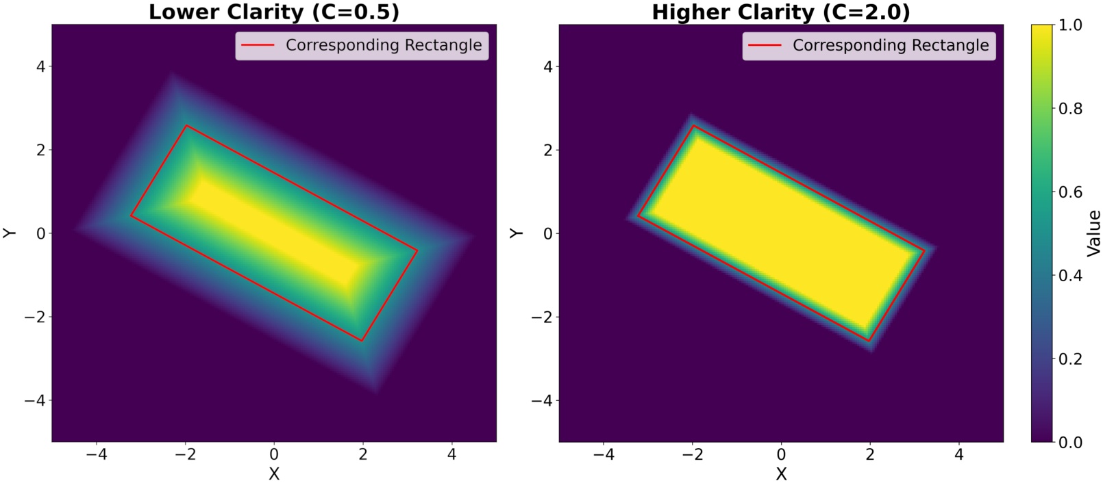
Figure 4.
Comparison of rectangle function with different sharpness parameters. Both plots show a rectangle with dimensions 6.0 × 2.5 and rotation angle 30°. Left: Lower clarity (C=0.5) produces smoother transitions. Right: Higher clarity (C=2.0) produces sharper edges. The heatmaps display the continuous function values ri,j, with the red outline showing the corresponding rectangle boundaries. The boundaries of the corresponding rectangle lie in the middle of the transition region
Merging operation
The merging operation is applied when two rectangles overlap or cover areas that can be more efficiently represented by a single rectangle. We proceed as follows:
Compute the average orientation θavg of the two rectangles, θ1 and θ2.
Create a new rectangle, oriented along θavg, that covers all vertices of the two input rectangles.
Compare the area of the merged rectangle Amerged with the sum of the areas of the two input rectangles A1 and A2. If
where c is a constant slightly larger than 1 (e.g., c = 1.05), then merge the two input rectangles into the newly calculated rectangle.
Deleting operation
The deleting operation removes rectangles whose area is below a predefined threshold Amin. This prevents small, insignificant rectangles from cluttering the representation.
Splitting operation In some cases, poor initialization can cause a single rectangle to cover multiple disconnected open spaces, especially in the presence of narrow obstacles like walls. When this occurs, the rectangle should be split into multiple smaller rectangles, each corresponding to a separate open space. We proceed as follows:
Identify if the rectangle spans across multiple regions separated by obstacles by using a region-growing algorithm to find connected components within the rectangle.
For each connected region, apply Principal Component Analysis (PCA) to the set of points within the region to find the main orientation of the space.
Use the principal PCA vector to orient a new rectangle that covers the region.
Replace the original rectangle with the newly calculated set of smaller rectangles.
4.6. Path Planning
Inside each rectangle, we use a simple boustrophedon path along the longer side of the rectangle. If the path encounters an obstacle, we use A* to find the shortest path that avoids that obstacle. Finally, we sequence the set of rectangles by solving a Traveling Salesman Problem (TSP) to find a near-optimal solution that visits all regions.
Sweeping along the longer axis of each rectangle is a deliberate design choice that prioritizes predictability and geometric efficiency:
Predictability in industrial settings: Boustrophedon paths along consistent axes produce deterministic, easily predictable trajectories. This is critical for industrial cleaning robots operating in shared human environments, where path predictability enhances safety and operational reliability.
Geometric efficiency of rectangular decomposition: Our segmentation algorithm naturally decomposes free space into rectangles (corridors, hallways). For such geometries, sweeping along the longer axis minimizes turning points and maximizes straight-line coverage segments, reducing execution time and energy consumption.
4.7. Implementation Details
The entire pipeline is implemented in Python 3. Input maps can be loaded from standard formats (e.g., image files or ROS-style occupancy grids). We use NumPy for array processing and OpenCV for image-based operations. For each map, the segmentation outputs a list of rectangles, which we store in a JSON file. The final coverage path is stored as an ordered list of (x, y) waypoints in the same JSON. We also generate plots of the map, rectangles, and path using Matplotlib for verification. This modular design makes it easy to modify or extend each step.
The optimization algorithm was implemented using the Keras library to facilitate automatic gradient calculation and parameter updates. We use the Adam optimizer [31] to improve convergence speed and stability of the segmentation process. The fitting process is set to run for 300 iterations, with merge, delete, and split operations performed every 30 iterations. The choice of these hyperparameters reflects a balanced trade-off between two competing objectives. First, the Adam optimizer leverages adaptive learning rates and momentum estimates to accelerate convergence and navigate the non-convex optimization landscape effectively. However, excessive iterations without structural modification can lead to sub-optimal local minima, as the gradient-based updates alone cannot escape geometrically inefficient rectangle configurations. Second, the merge, delete, and split operations are crucial for escaping such local minima by restructuring the solution space. Performing these operations too frequently (e.g., every iteration) introduces instability, as the optimizer has insufficient time to refine parameters before the topology changes. Conversely, performing them too infrequently reduces their effectiveness in improving the overall segmentation quality.
5. Simulation and results
We evaluated our method on multiple test environments recorded in warehouses, shopping malls and production facilities. Test environments have different dimensions ranging from 2109 × 1221 px to 6159 × 5079 px. All experiments were run on a standard desktop (Intel Core i7 CPU, 16 GB RAM). Our software environment was Python 3.11.
5.1. Benchmark Algorithms
To evaluate the advantages of the proposed method, results are compared to three benchmark planning methods:
Boustrophedon: A classical coverage path algorithm that generates zigzag paths. [3]
Neural network: The method uses a topologically organized neural network, governed by shunting dynamics based on Hodgkin and Huxley’s equation, to autonomously generate collision-free, complete coverage paths for cleaning robots in dynamic environments through local neural interactions and previous robot positions. [32]
Energy functional: The coverage path planning method directs the robot to systematically explore a room by following a grid of observation points, selecting each next point based on an energy function that balances travel efficiency, smooth navigation, and area coverage while adapting to dynamic obstacles. [33]
The implementations of the benchmark algorithms were sourced from the open-access library https://github.com/ipa320/ipa_coverage_planning [8].
5.2. Performance Metrics
For each method we measured average values of the metrics described above. The values are presented in Table 1.
Table 1.
Summary of results for different methods
| Method | avg. Length per m2 | avg. Coverage | avg. Curvature per m2 | avg. Time per m2 |
|---|---|---|---|---|
| Boustrophedon [3] | 2.861 | 0.8713 | 1.001 | 6.893 |
| Neural Network [32] | 5.110 | 0.8713 | 1.880 | 12.907 |
| Energy Functional [33] | 2.563 | 0.9831 | 2.520 | 10.863 |
| Gradient-Based Segmentation | 2.094 | 0.8664 | 0.474 | 4.594 |
For every algorithm, the following parameters were used. Parameters were selected based on real cleaning robot data. Same set of parameters are used on our proposed Efficient Coverage Path Planning via Gradient-Based Rectangular Segmentation method and three benchmark methods.
Robot radius: 0.4 m
Coverage radius: 0.32 m
Time calculation parameters:
– Maximum linear velocity: 0.5 m/s
– Maximum angular velocity: 1.0 rad/s
– Maximum linear acceleration: 0.3 m/s2
– Maximum angular acceleration: 0.5 rad/s2
– Maximum linear deceleration: 0.3 m/s2
– Maximum angular deceleration: 0.5 rad/s2
Overall, the proposed rectangular segmentation yielded smoother and more efficient coverage paths. The path visuals (see Figure 5) show clean back-and-forth sweeps covering each region. Our method outperformed the benchmarks in average path length per m2 giving overall shorter paths, significantly smaller curvature per m2 meaning paths are simpler and the robot can achieve higher average velocity. Time per m2 is also significantly smaller than other algorithms due to the shorter and simpler paths. The algorithm maintained good coverage (comparable to the boustrophedon benchmark).
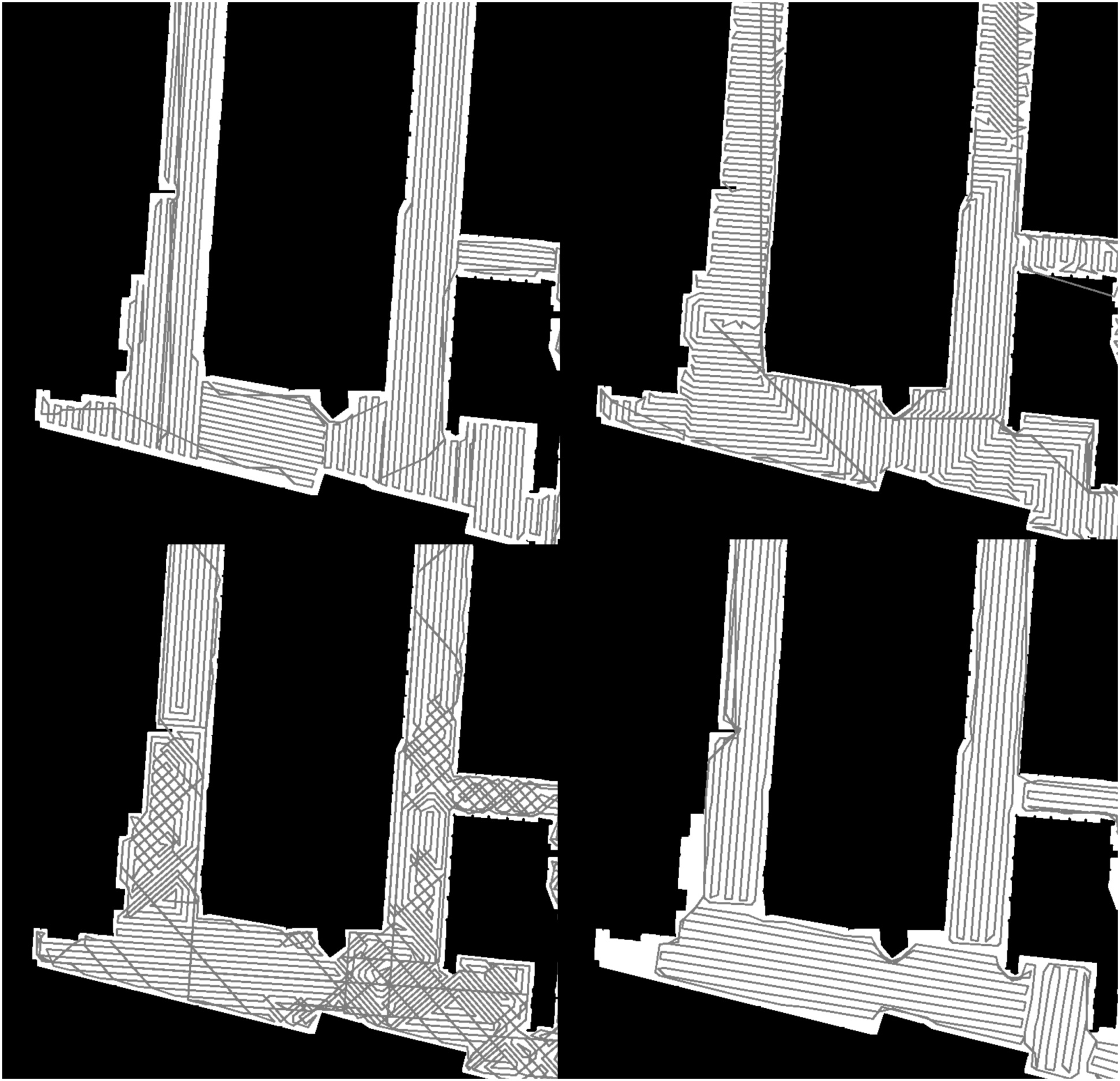
Figure 5.
Visual comparison of coverage paths generated by different algorithms. Boustrophedon (top left), Energy Functional (top right), Neural Network (bottom left), Gradient-Based Rectangular Segmentation (bottom right)
5.3. Sensitivity to Coverage Weighting Parameter
To quantify the effect of the weighting parameter α introduced in the weighted objective function, we evaluated three representative values on our benchmark maps:
α = 1: Coverage of 86.64% with 4.59 s/m2 execution time
α = 1.5: Coverage of 89.98% with 4.69 s/m2 execution time
α = 3.0: Coverage of 92.97% with 5.22 s/m2 execution time
α = 10.0: Coverage of 93.31% with 5.50 s/m2 execution time
These results demonstrate a clear trade-off between coverage completeness and execution efficiency. Higher values of α lead to better coverage but increase path complexity and execution time, as rectangles are pushed to cover marginal areas at the cost of geometric regularity. For the experiments reported in this paper, we used α =1, which provides a balanced compromise between coverage quality and efficiency. However, applications requiring maximum coverage (e.g., critical cleaning tasks in sterile environments) may benefit from higher values despite the increased execution time. Further improvements, such as reinitializing new rectangles in uncovered regions at a later stage of the optimization, remain future work.
6. Conclusion
We have presented a new coverage path planning framework that uses gradient-based rectangular segmentation of the environment. By partitioning the map into axis-aligned rectangles adapted to obstacle boundaries, our method enables simple back-and-forth sweep coverage in each zone. This leads to coverage paths that are smooth, easy to track, and efficient in terms of travel distance.
The experimental results demonstrate that our approach improves the efficiency of the Boustrophedon path planning algorithm. Notably, the proposed method achieves shorter paths with fewer turns while maintaining high coverage of the target area. This highlights the robustness and scalability of our solution, making it particularly useful in industrial and commercial robotics applications.
Segmentation of the map enables easy manual modifications of the paths. Another advantage is that path of the robot is easier to predict, which is important in environments with a human traffic.
Despite these promising results, several areas for future work remain. Firstly, the computational cost of the segmentation process, particularly during gradient descent, could be further reduced. By employing more sophisticated optimization techniques, such as metaheuristic approaches, may enhance the computational performance. The low coverage of the method can be improved by creating planning paths in areas not covered by the algorithm. Additionally, rectangle function can be modified to avoid local minima.
Another avenue for future research involves exploring more sophisticated strategies for path planning within segmented rectangles. While the current approach employs simple Boustrophedon paths, more advanced path-planning methods could further improve the efficiency of the robot’s movement, especially in cluttered environments.
Our method provides a significant step forward in the field of Coverage Path Planning by combining map segmentation, optimization, and efficient path generation. Future research should focus on enhancing computational efficiency, robustness to real-world conditions to improve system performance further. We believe that these developments will contribute to the broader adoption of autonomous robotic solutions in various sectors, including manufacturing, logistics, and cleaning services.