

1. Introduction
Nowadays, the demand for mobile robots is rising as they have the potential to free humans from repetitive, dangerous, and labor-intensive tasks [1,2,3,4]. In industries such as manufacturing, logistics, and healthcare [5, 6], mobile robots are increasingly utilized for tasks like assembly line work, warehouse management, and patient transport. By taking over these duties, mobile robots not only enhance efficiency and productivity but also reduce the risk of injuries and allow human workers to focus on more complex and creative activities. Thanks to their remarkable omni-directional mobility, four Mecanum-Wheeled Mobile Robots (FMWMRs) have garnered significant interest across various sectors, including military and industrial applications [7,8,9]. With special design of mecanum wheel, it allows the robots to navigate confined and intricate spaces with ease, making them highly useful in various fields such as industrial automation, warehouse operations, and search and rescue efforts [10]. Through the independent control of speed and direction for each wheel, this configuration enables FMWMRs to maneuver instantly in any direction from any starting orientation, eliminating the requirement for pre-orientation. As a result, compared to conventional platforms, these vehicles have excellent mobility and are well-suited for operations in confined places or crowded areas [7].
However, achieving accurate trajectory tracking and motion control of such platforms remains a challenge due to parameter uncertainties, non-linearities, external disturbances and the need for robust control strategies. These factors can further degrade the control performance. As a result, there are many problems that need to be solved when implementing a Mecanum robot project, such as control algorithm problems, position and rotation angle determination problems and so on [9, 11,12,13,14]. Many research works have been conducted to develop and implement different kinds of control techniques, such as: PID control [15, 16], backstepping control [17], sliding mode control [18], intelligent control based on neural networks [19, 20].
Fuzzy PID controllers are applied in various fields, including robotics, industrial automation, and process control, where system conditions are constantly changing and require adaptive control strategies. A Fuzzy PID controller combines the principles of a conventional PID (Proportional-Integral-Derivative) controller with fuzzy logic to improve performance in systems with non-linearity, uncertainties, or varying dynamics. Compared to conventional PID controllers, the Fuzzy PID controller demonstrates superior characteristics such as better handling of non-linearities, robustness in conditions of system uncertainty, and effective adaptation to dynamic environments without needing a precise mathematical model. Thanks to these advantages, Fuzzy PID controllers have been extensively investigated in numerous research studies [16, 21,22,23,24,25,26]. In [16, 21,22,23, 27], the Fuzzy PID controller was employed to control the mobile robot in condition of uncertainty factors such as friction, disturbance, and the robot’s nonlinearity. While in [24,25,26], the fuzzy PID is applied in some other fields such as a permanent magnet synchronous motor, tranformer coil temperature or active suspension.
For effective trajectory tracking and motion control in FMWMRs or mobile robots, precise localization and heading angle estimation need to be determined. Robot positioning and heading angle fusion methods play a crucial role in enhancing the accuracy and reliability of robotic navigation systems. Common positioning approaches include GPS [2], inertial sensors - IMU [28, 29], and vision systems [28, 30], LiDAR [31,32,33]. Especially, for indoor robot positioning, various methods have been explored, including IMU (Inertial Measurement Unit) and its sensor fusion techniques, ultrasonic sensors, infrared sensors, vision-based systems, radio frequency technologies, and LiDAR. The technologies, along with the advantages and drawbacks of each method, of these methods are discussed in [31, 34, 35]. Additionally, various fusion algorithms, such as Kalman filters [36], hidden Markov model [37, 38] or Bayesian estimation [2, 28, 39,40,41], are utilized to merge sensor data and reduce errors. Besides, to measure the robot’s orientation, the IMU, which combines a magnetometer, accelerometer, and gyroscope, is extensively used. Well-known methods for calculating the heading angle with an IMU include the Complementary filter [29], Extended Kalman filter [28, 41, 42], Madgwick filter [43, 44] and Mahony filter [45]. However, IMUs have intrinsic limitations, including drift overtime due to cumulative sensor errors and vulnerability to external environmental factors like magnetic interference. To address these drawbacks, sensor fusion methods are employed to combine IMU data with other sensor inputs, enhancing overall reliability and performance.
In this paper, a comprehensive control system is investigated to achieve precise tracking control of FMWMRs. The controller structure is composed of a Fuzzy logic controller for orientation control and a Fuzzy-PID controller for position control. Through this integration, the trajectory tracking and motion control performance of FMWMRs are significantly improved. Velocities along the x and y axes are computed by the Fuzzy-PID controller based on position error and its derivative, while angular velocity is determined by the Fuzzy logic controller using the error and derivative of the heading angle. These computed velocities are subsequently utilized as inputs to inverse kinematic equations to derive the necessary wheel velocities. System nonlinearities and uncertainties are effectively managed and compensated by the fuzzy rule base through expert tuning.
To evaluate the control performance, extensive simulations were conducted in the Matlab/Simulink environment. The PID and Fuzzy controllers were also implemented to assess the superiority of the Fuzzy-PID approach. Additionally, a real-life FMWMR prototype was constructed to verify the effectiveness of the proposed controller under practical conditions. For obtaining the FMWMR’s position and heading angle, a vision technique based on ArUco markers [46, 47] is employed. However, challenges such as sensitivity to lighting conditions and slow response rates are encountered with this approach. To address these limitations, an IMU is integrated with the ArUco marker detection results using a complementary filter [29], thereby improving the response and accuracy of the heading angle estimation. The overall of control approach and sensor fusion methodology can be illustrated in a comprehensive way as shown in Figure 1. The simulation and experimental results demonstrate the superiority of the proposed control system in achieving precise trajectory tracking and motion control for FMWMRs in both simulation and real-world scenarios.
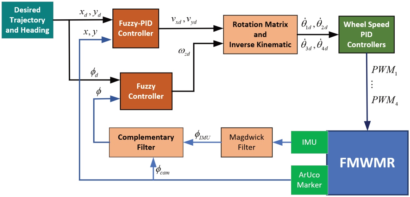
Figure 1.
Overall structure of the proposed control system
The subsequent parts of this paper are organized as follows: Section II summarizes the mathematical model of a FMWMR. Section III details all the steps in Fuzzy and Fuzzy-PID design process. The method of positioning and orientation determination by sensor fusion is then illustrated in Section IV. Simulation, experiment results and discussion are shown in Section V. Finally, Section VI concludes our research and provides future directions for development.
2. Mathematical model
In this research, the mathematical model of FMWMR in [48] is used. In which, the kinematic model and dynamic model of FMWMR can be summarized as:
The robot kinematic model:
The robot’s inverse kinematic model:
In world frame – as shown in Figure 2, the robot motion is determined as:
where: is a vector of robot motion in inertia frame; is a vector robot motion in robot frame; is a vector of rotation angle of robot wheels; is robot heading angle; rw is radius of mecanum wheel.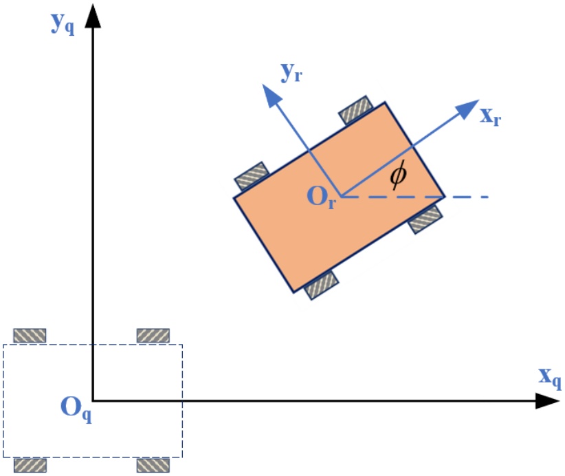
Figure 2.
Robot in world frame and robot frame
J is geometry matrix of robot; J+ is inverse matrix of J
a and b are haft of width and length of the robot flatform; ℜ(ϕ) is frame convert matrix, which is determined as:
The dynamic model of FMWMR is determined as:
where: is a vector of applied torque generated by robot wheel motors; ; with represents the static friction on mecanum wheels.3. Controller Design
For FMWMRs to operate well, trajectory tracking and motion control need a resilient and flexible control system that can deal with uncertainties, non-linearities, and external disturbances. A hierarchical of control architecture that includes a fuzzy-PID controller for position control with a fuzzy logic controller for orientation control is investigated in order to overcome these issues. While the Fuzzy-PID controller is responsible for regulating the robot’s position, the Fuzzy logic controller is designed to control the robot’s heading angle, guaranteeing precise orientation tracking. The overall block diagram of the control system is illustrated in Figure 3. Each controller’s design process will be detailed in the following subsections, beginning with the fuzzy controller used for orientation control.
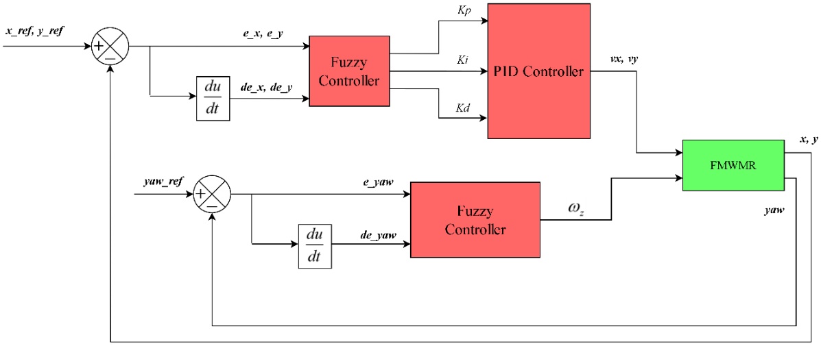
Figure 3.
Block diagram of the control system
3.1. Fuzzy logic controller for orientation control
To control the robot’s orientation, a fuzzy logic controller is designed with two inputs and one output, as shown in Figure 4. The inputs consist of the heading angle error between the desired orientation and the robot’s orientation ( ) and its derivative ( ). The output is the desired angular velocity of the robot. Since the inputs and output of the fuzzy logic controller operate within different physical ranges, significant time is required to adjust the fuzzy logic for each variable in varying situations. To address this, in this research, all inputs and outputs of the fuzzy controller are normalized to the standard range [-1, 1] using normalization gains. This normalization simplifies the formulation of the fuzzy rule base and provides flexibility in adjusting input and output ranges during performance evaluation and tuning. By adjusting the normalization gains, the expected range can be modified, enabling the designed membership functions to automatically adapt to the new range without requiring a complete redesign.
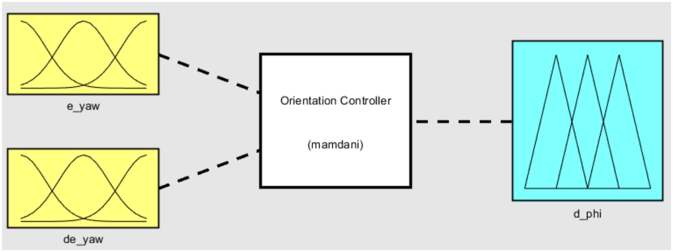
Figure 4.
Inputs and output of heading angle Fuzzy logic controller
Fuzzification
The design approach for the heading angle fuzzy controller begins with fuzzification. In this step, the crisp input values are converted into fuzzy sets using membership functions. Trapezoidal and triangular membership functions are used in this design due to their simplicity and ability to clearly represent the input and output spaces.
Based on experience from simulation and experiment results, the fuzzy inputs are fuzzified using seven membership functions: BN (Big Negative), MN (Medium Negative), SN (Small Negative), ZE (Zero), SP (Small Positive), MP (Medium Positive), and BP (Big Positive). The distribution of the membership functions of each input is illustrated in Figure 5 and Figure 6.
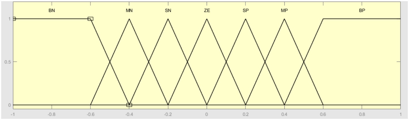
Figure 5.
Design of membership functions for heading angle error’s fuzzy input
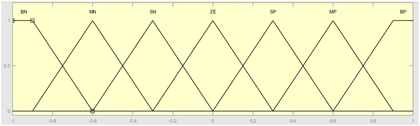
Figure 6.
Design of membership functions for derivative of heading angle error fuzzy input
Similarly, for the fuzzy output, the angular velocity is fuzzified using seven membership functions: BN (Big Negative), MN (Medium Negative), SN (Small Negative), ZE (Zero), SP (Small Positive), MP (Medium Positive), BP (Big Positive). The distribution of these membership functions is illustrated in Figure 7.
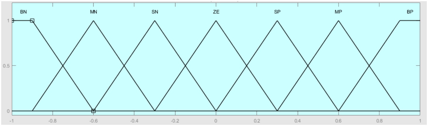
Figure 7.
Design of membership functions for angular velocity fuzzy output
The normalization gains for inputs and outputs of orientation controller are selected and presented as Table 1.
Fuzzy Rule Base
The fuzzy rule base comprises a set of IF-THEN rules that determine the appropriate control action based on the linguistic values of the input variables. The rules consider the combination of error and rate of change of error to determine the appropriate velocities for the robot. Each rule specifies the linguistic values of the inputs and the desired linguistic value of the output. These fuzzy rules were derived from the experience of numerous simulations and experiments, aiming to achieve the most effective control system as shown in Table 2.
Fuzzy Inference System
Once the fuzzy rule base is established, the fuzzy inference system combines the fuzzy rules with the fuzzified input values to determine the appropriate control action. In this paper, the Mamdani’s Fuzzy Inference method with Max–Min composition is applied. It involves combining the minimum of the degrees of membership for each rule during aggregation and considers the maximum value of these minimum values during defuzzification.
Defuzzification
The defuzzification process converts the fuzzy output into a crisp output value of the angular velocity. In this implementation, the Center of Gravity (COG) method is leveraged for defuzzification, which calculates the centroid of the aggregated output fuzzy set.
3.2. Fuzzy-PID controller for position control
This section presents the use of fuzzy logic to tune the parameters of PID controllers for trajectory tracking along the x and y axes. Two fuzzy PID controllers are independently designed for each axis. The structure of the fuzzy system, shown in Figure 8, includes two inputs (position error and its derivative) and three outputs (the PID controller gains). Similar to the orientation controller, all the inputs and outputs of fuzzy logic controller in this section are designed in a normalized range of [-1, 1] with inputs and [0, 1] with outputs. The details of the fuzzy tuning process are described as follows:
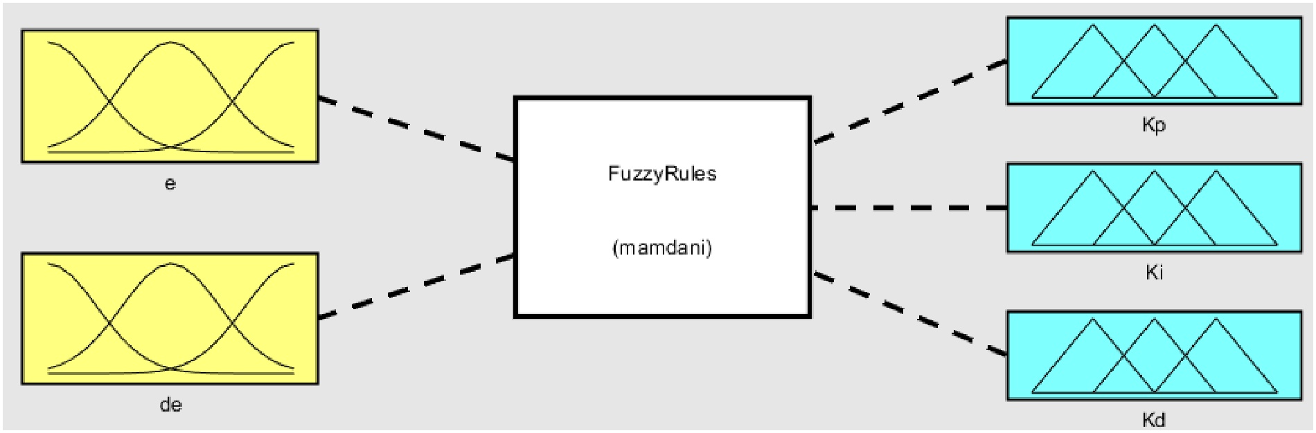
Figure 8.
Structure of inputs and outputs Fuzzy logic design
For the inputs of fuzzy logic, each tracking position error along each axis ( or ) is fuzzified using five membership functions: NB (Negative Big), NS (Negative Small), ZE (Zero), PS (Positive Small), and PB (Positive Big). Similarly, the derivative of the position tracking error ( or ) is fuzzified using the same five membership functions: NB (Negative Big), NS (Negative Small), ZE (Zero), PS (Positive Small), and PB (Positive Big). Figure 9 and Figure 10 illustrate the membership functions fuzzy logic inputs. The normalization gains are set to 0.02 for the position error and 0.04 for the error derivative.
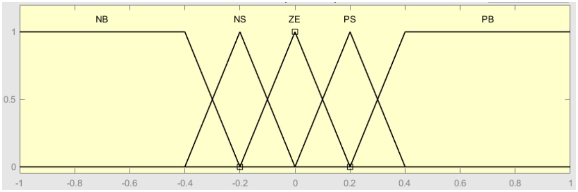
Figure 9.
Position error’s membership function
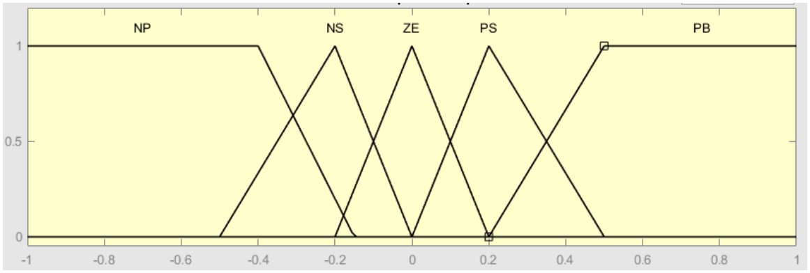
Figure 10.
Derivative of position error’s membership function
The fuzzy outputs include three parameters of PID controller Kp, Ki and Kd, which are normalized in range of [0, 1]. These output values are fuzzified using five membership functions: S (Small), MS (Medium Small), M (Medium), MB (Medium Big), B (Big). The membership functions of these outputs are designed similarly as illustrated in Figure 11.
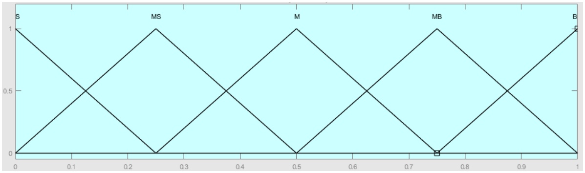
Figure 11.
Membership function for fuzzy outputs - the PID normalized gains
Based on the experience through extensive simulations and experiments, for best control performance, PID controller gains are chosen to vary in ranges of: , , . In fuzzy outputs, these parameters are normalized into the range of [0, 1] by equation (6).
where Kx stands for the reality PID gains Kp, Ki or Kd; and stands for the normalized PID gains (Fuzzy outputs) , or . From (6), the value of PID parameter gains can be calculated from fuzzy output by equation (7).Thus, as a result, the value of Kp, Ki or Kd can be detailed as: ; ; .
Based on tuning and evaluation of control of performance, the rule base for three outputs of the fuzzy logic is established in a similar manner and is illustrated as in Table 3.
Table 3.
Fuzzy rule base for controlling Kp, Ki, Kd
| e | ||||||
| NB | NS | ZE | PS | PB | ||
| de | ||||||
| NB | B | MB | S | S | M | |
| NS | B | M | S | MS | MB | |
| ZE | MB | MS | S | MS | MB | |
| PS | MB | MS | S | M | B | |
| PB | M | S | S | MB | B | |
To determine the fuzzy outputs, the Mamdani Fuzzy Inference Method with Max–Min composition and COG defuzzification, is applied. This method is identical to the design process used for the fuzzy controller in orientation control mentioned earlier.
4. Experiential Setup and Heading Angle Fusion Technique
4.1. Experimental Setup
The structure of the experimental control system is illustrated in Figure 12. In this setup, the vision-based ArUco marker detection method and trajectory tracking Fuzzy PID controllers are executed on a laptop computer. The ATmega 2560 is responsible for calculating the robot’s orientation (Magdwick and Complementary filters), executing the heading angle Fuzzy controller, and managing the wheel speed PID controllers. Communication between the laptop and the ATmega 2560 is facilitated via a Bluetooth module (HC-05). The block diagram showing the functional blocks of the real-world implementation for mecanum robot control is presented in Figure 13.
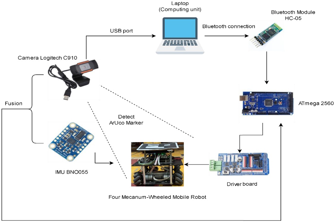
Figure 12.
Structure of the experimental execution
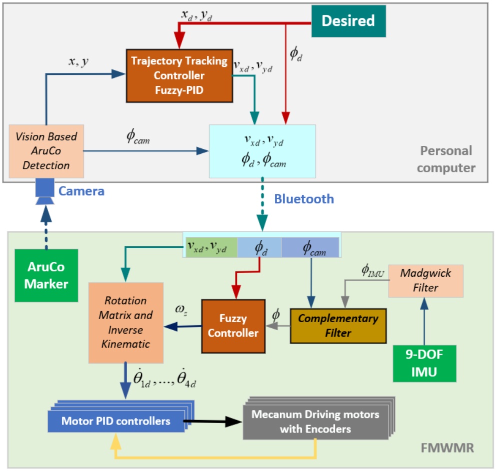
Figure 13.
Overall block diagram of real-life FMWMR control
4.2. Heading Fusion Technique
Accurate heading angle estimation is crucial for precise trajectory tracking and motion control in FMWMRs. To achieve reliable and robust heading angle estimates, a sensor fusion approach that combines data from a camera-based localization system and an Inertial Measurement Unit (IMU) is investigated.
An ArUco marker affixed to the robot is detected by the camera-based localization system, employing an overhead camera. Through analysis of the marker’s pose, the system establishes the robot’s position and orientation in the global coordinate system. Despite its utility, ArUco marker detection is susceptible to limitations such as sensitivity to lighting conditions and a slow detection… To mitigate these constraints, IMU data are concurrently utilized to augment the accuracy of heading angle detection. The IMU integrates signals from accelerometers, magnetometers, and gyroscopes, facilitating the Madgwick filter [44] in estimating a drift-free and responsive heading angle. Subsequently, the robot’s heading angle is determined by combining data from both the camera and IMU using the complementary filter [43]. Here, the IMU supplies rapid angle variations via a high-pass filter, complemented by the camera’s provision of slower variations through a low-pass filter. Figure 14 illustrates the complementary filter integration.
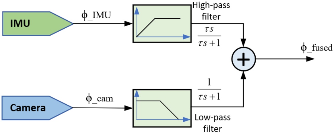
Figure 14.
Block diagram of heading angle fusion using complementary filter
The mathematical models of the complementary filter using first order filter in both Laplace and Z domains are expressed in Eq. (8) and (9), respectively.
Consequently, the final heading angle can be computed from the IMU and camera as equation (10).
where: is fused heading angle (degree); is heading angle from the camera (degree); is heading angle from the IMU (degree); ; Ts is sampling time; τ is low-pass filter time constant which is chosen as 1s in this research.Figure 15 presents a comparison of the IMU response, vision detection, and the fusion results. Figure 15a highlights the IMU response obtained from Magdwick filter, showing significant detection errors due to accumulation effects and environmental uncertainties. In contrast, Figure 15b displays the vision detection result from the Aruco marker. This result is shown under the worst conditions, where light variability and pixel errors heavily impact detection accuracy. Finally, Figure 15c illustrates the outcome of the complementary filter. This fusion response demonstrates the advantages of the fusion method, effectively reducing the drawbacks of both the IMU and vision sensors. The enhanced heading angle from the fusion can be applied to experimental control in further sections.
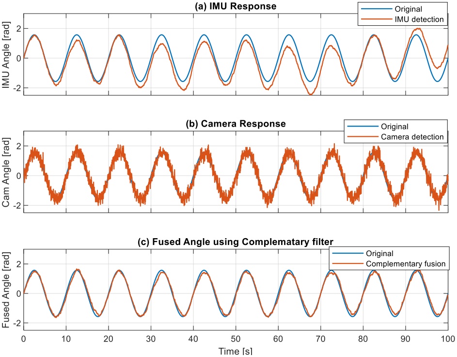
Figure 15.
Heading angle detection using IMU, Vision- ArUco marker and Complementary filter fusion
5. Results and Discussion
To evaluate the performance of the proposed control system and sensor fusion approach, extensive simulations and real-world experiments are conducted. This section presents and analyzes the results obtained from both the simulation studies and the experimental validation.
5.1. Simulation Results
Simulation results using Matlab/Simulink environment are performed to compare the tracking performance of three control strategies: PID, Fuzzy, and Fuzzy-PID. The simulations were carried out under various scenarios, including desired position, rectangular reference trajectory and eight-shaped reference trajectory.
For the desired position scenario, the response and error plots are illustrated in Figure 16 and Figure 17, respectively. Analysis of the response plots demonstrates that the Fuzzy controller achieves the fastest response in reaching the desired x and y positions. In comparison, the PID controller responds slightly slower and exhibits some oscillation before settling while both Fuzzy and Fuzzy-PID controllers show quick and smooth convergence to the desired yaw angle. Despite the differences in response times, all three controllers successfully converge to the target position and heading angle with minimal steady-state error.
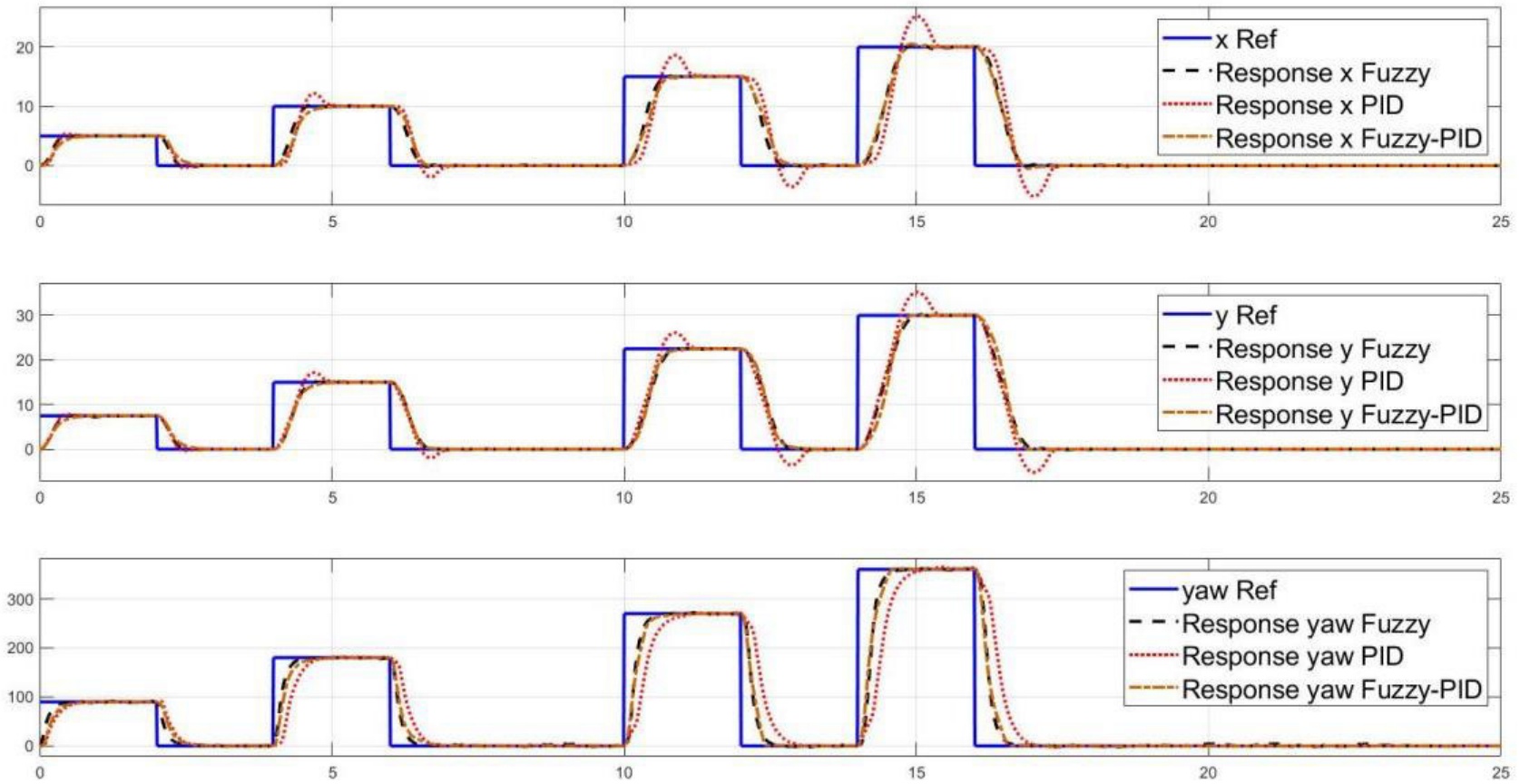
Figure 16.
Position responses with respect to multi-step reference in simulation
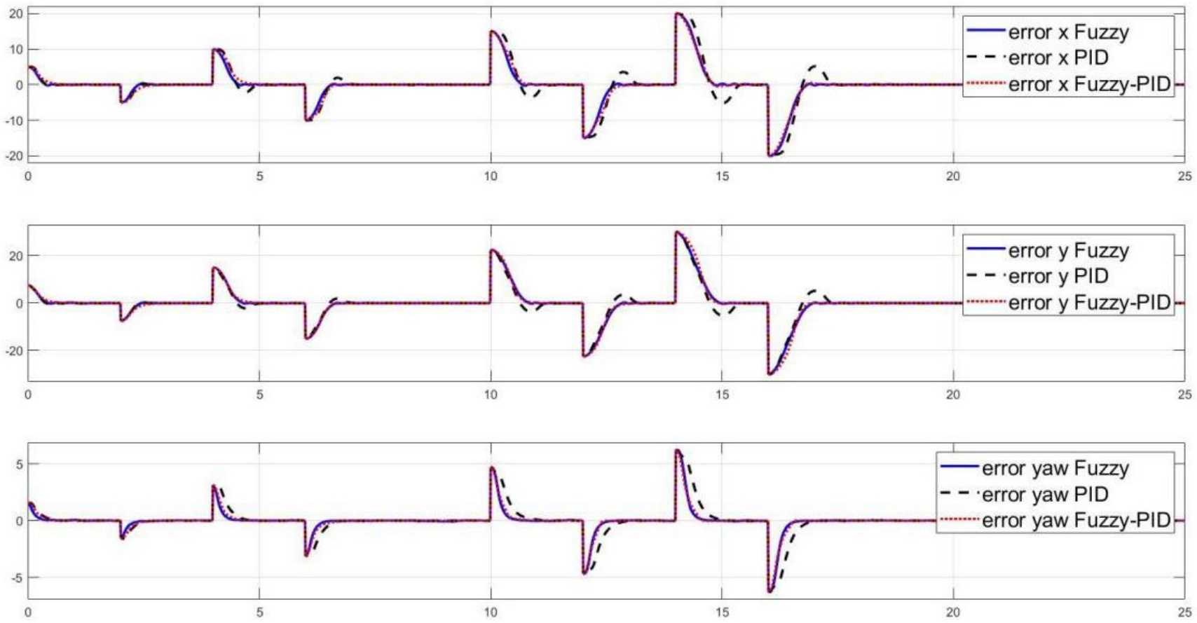
Figure 17.
Position control errors with respect to multi-step reference in simulation
Next, the rectangular path trajectory scenario control results are presented in Figure 18 to Figure 20, respectively. From the robot’s path in the x-y plane, it is obvious that the Fuzzy-PID controller performs the best, attaining the smoothest and most accurate tracking (Figure 18). The Fuzzy-PID controller maintains the lowest error values in all dimensions (x, y, and heading angle), as shown by the error plots (Figure 20), which validate its improved tracking accuracy. Though having somewhat greater deviations and error magnitudes than the Fuzzy-PID controller, the fuzzy controller also shows good tracking capabilities. On the other hand, the tracking performance of the PID controller is less accurate, exhibiting more pronounced oscillations, undershoots, and overshoots, especially at the rectangle’s corners.
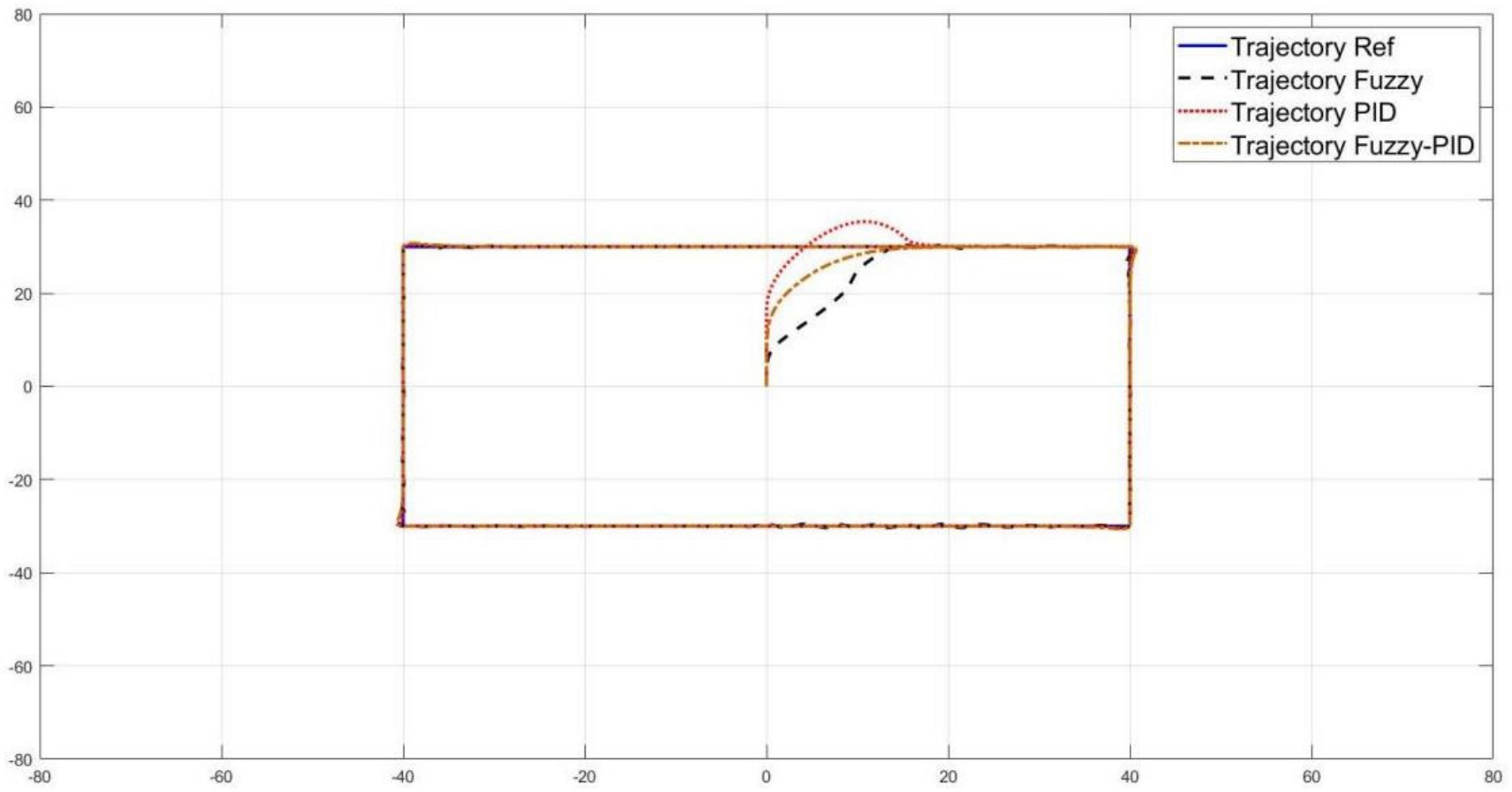
Figure 18.
Rectangular path trajectory tracking control responses in simulation
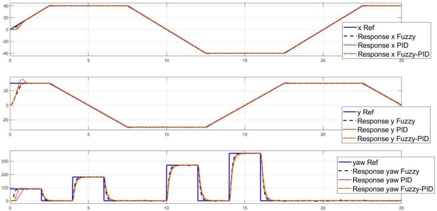
Figure 19.
Control responses with respect to rectangular path trajectory tracking control in simulation
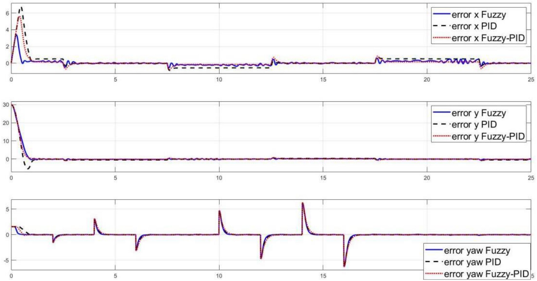
Figure 20.
Control errors with respect to rectangular path trajectory tracking control in simulation
Besides, an eight-shaped trajectory was utilized to assess the controllers’ performance further in Figure 21 to Figure 23. This difficult maneuver tests the robot’s capacity to manage abrupt direction changes and sharp turns. All three controllers are able to follow the intended 8-shaped path, as seen by the trajectory tracking plot (Figure 21), with the Fuzzy-PID controller adhering to the reference trajectory that is closest. The Fuzzy-PID controller outperforms the others, as seen by the error plots (Figure 23), which show the lowest x, y, and heading angle error magnitudes. Whereas the PID controller displays greater error magnitudes, the fuzzy controller maintains very low error values.
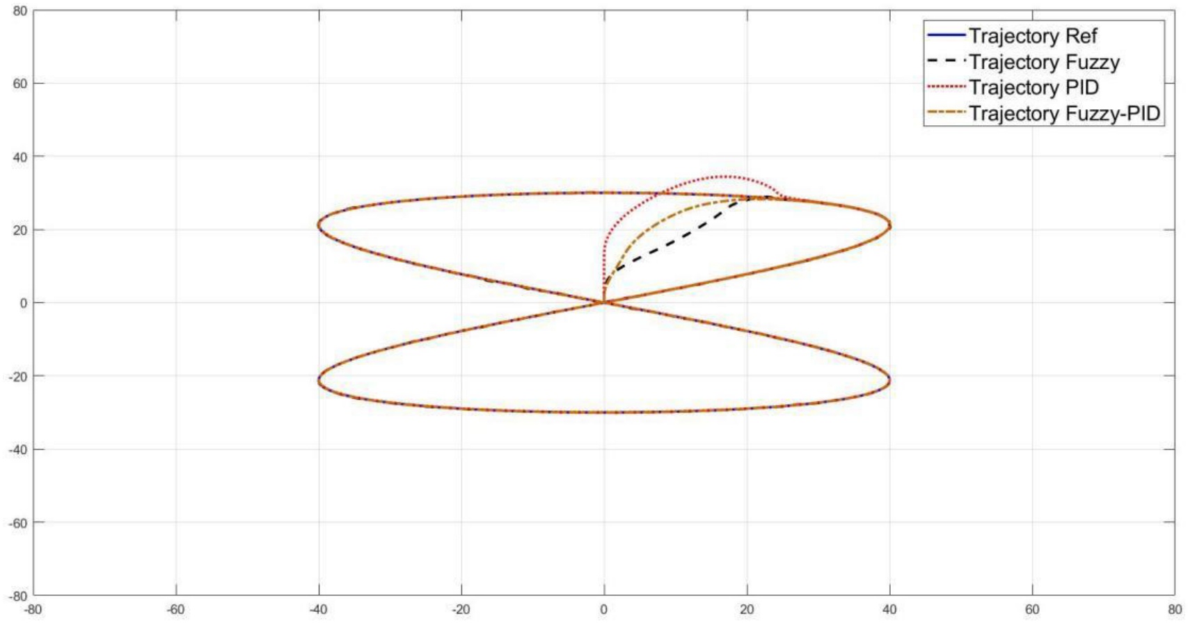
Figure 21.
8-shaped path trajectory tracking control results in simulation
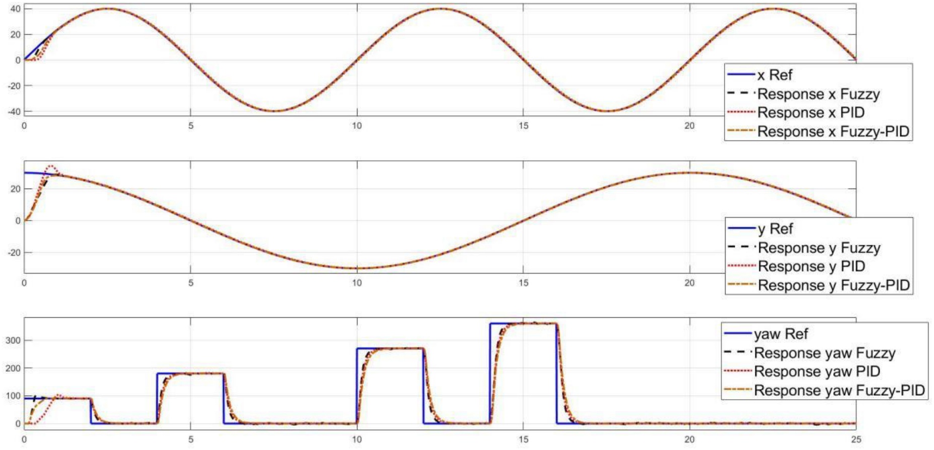
Figure 22.
Control responses with respect to 8-shape path trajectory tracking control in simulation
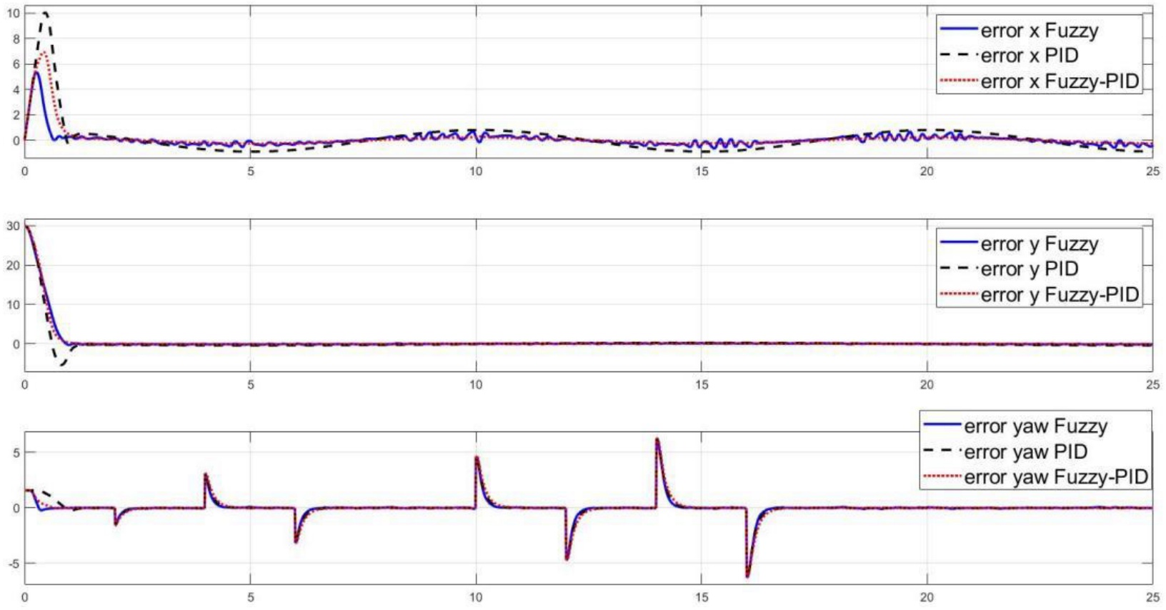
Figure 23.
Control response error with respect to 8-shape path trajectory tracking control in simulation
Based on simulation results, the control performances of three controllers are evaluated. Table 4 and Table 5 present the comparison results of these controllers. These tables display each controller’s x-position and yaw responses across four criteria: Overshoot, rise time, steady-state error, and settling time. The results demonstrate that the Fuzzy-PID controller exhibits superior performance, characterized by zero overshoot, minimal steady-state error, and a fast response.
Table 4.
Comparison among the x responses of each controllers
| Setpoint | Parameters | PID | Fuzzy | Fuzzy-PID |
|---|---|---|---|---|
| 5 | Overshoot (%) | 8.02 | 5.07 | 0 |
| Rise time (s) | 0.31 | 0.24 | 0.37 | |
| Steady state error | 0.0273 | 0.0089 | 0 | |
| Settling time (s) | 0.63 | 0.5 | 0.77 | |
| 10 | Overshoot (%) | 21.8 | 1.43 | 0 |
| Rise time (s) | 0.26 | 0.34 | 0.44 | |
| Steady state error | 0.0318 | 0.006 | 0 | |
| Settling time (s) | 1.01 | 0.55 | 0.87 | |
| 15 | Overshoot (%) | 24.07 | 2.09 | 0 |
| Rise time (s) | 0.31 | 0.22 | 0.47 | |
| Steady state error | 0.0585 | 0.0007 | 0 | |
| Settling time (s) | 1.19 | 0.66 | 0.74 | |
| 20 | Overshoot (%) | 26.05 | 0.8 | 2.05 |
| Rise time (s) | 0.35 | 0.48 | 0.51 | |
| Steady state error | 0.0722 | 0.0002 | 0.0002 | |
| Settling time (s) | 1.36 | 0.81 | 0.79 |
Table 5.
Comparison among the yaw responses of each controllers
| Setpoint | Parameters | PID | Fuzzy | Fuzzy-PID |
|---|---|---|---|---|
| 90 | Overshoot (%) | 1.24 | 1.11 | 0.06 |
| Rise time (s) | 0.39 | 0.25 | 0.33 | |
| Steady state error | 0.2911 | 1.23 | 0.07 | |
| Settling time (s) | 0.93 | 0.61 | 0.69 | |
| 180 | Overshoot (%) | 0.55 | 0.27 | 0 |
| Rise time (s) | 0.4 | 0.26 | 0.34 | |
| Steady state error | 1.167 | 0.386 | 0.32 | |
| Settling time (s) | 0.78 | 0.48 | 0.72 | |
| 270 | Overshoot (%) | 0.4 | 0.39 | 0 |
| Rise time (s) | 0.52 | 0.25 | 0.31 | |
| Steady state error | 1.48 | 0.756 | 0.126 | |
| Settling time (s) | 1 | 0.55 | 0.63 | |
| 360 | Overshoot (%) | 1.2 | 0.03 | 0 |
| Rise time (s) | 0.54 | 0.27 | 0.37 | |
| Steady state error | 2.76 | 1.35 | 0.57 | |
| Settling time (s) | 0.94 | 0.56 | 0.54 |
Overall, the Fuzzy-PID controller has the best overall performance for both the x and yaw responses, offering exceptional stability, precision, and convergence speed, according to the provided data. The Fuzzy controller is a dependable option since it provides a decent balance between stability and responsiveness. With greater overshoot, slower response times, and larger steady-state errors than the other two controllers, the PID controller performs less well than the other two. From the obtained simulation results, we proposed a novel control approach for the FMWMR model in a real-life system. The experimental results will be discussed in detail in the following section.
5.2. Experimental Results
The superior performance of the Fuzzy PID controller is demonstrated by the simulation results. In this subsection, this controller will be employed and experimental results will be presented under various conditions. The performance of the control system will be investigated in different scenarios, including desired position, elliptical trajectory, rectangular trajectory, circular trajectory, and eight-shaped path trajectory. Furthermore, the robustness and tracking quality of the controller will be verified under a loaded condition of 2.5 kg. The examination of the control system’s tracking accuracy and path-following capability will be prioritized, with the unloaded condition applied specifically to the evaluation of the circular trajectory and eight-shaped path trajectory scenarios.
5.2.1. Desired position control scenario
In this experiment, the robot is set to move to the target position with coordinates x = 30cm, y = 30cm, and a yaw angle of 60 degrees. The control results are illustrated in Figure 24 to Figure 27. Figure 24 depicts the robot’s positional response in terms of x and y coordinates as well as yaw angle. It is evident that the robot reaches the target position within three seconds without any overshoot, while the yaw angle takes six seconds to stabilize. The steady-state error is nearly zero. The gains of the PID controllers are adjusted online and visualized in Figure 26 and Figure 27. Additionally, the effect of a 2.5kg load is examined in this scenario, revealing that the designed controller can adapt effectively to changes in load. The control performance remains consistent with that of the unloaded condition.
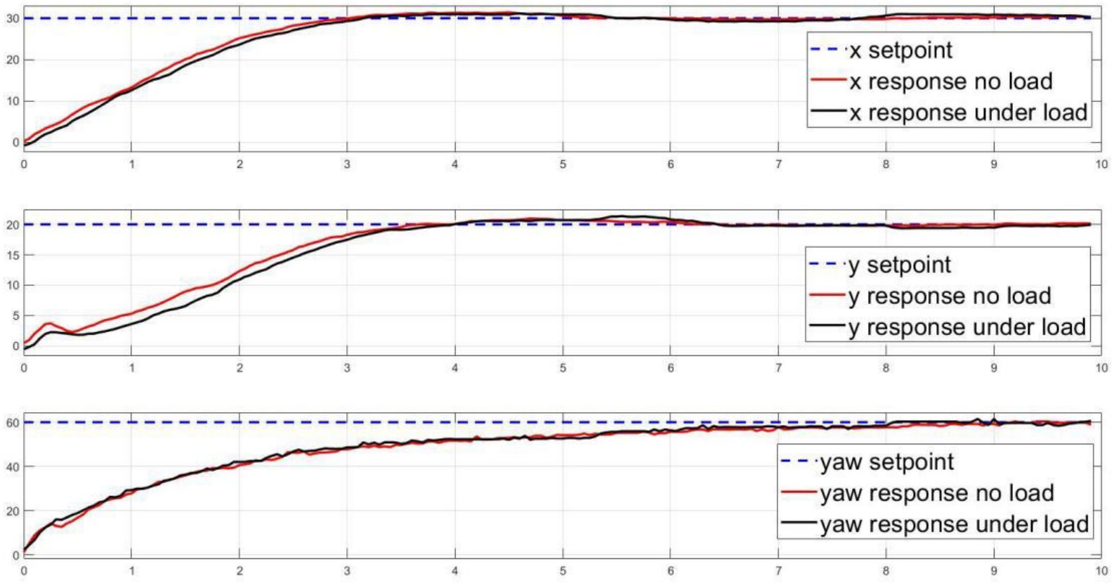
Figure 24.
Responses of robot with respect to target setpoint
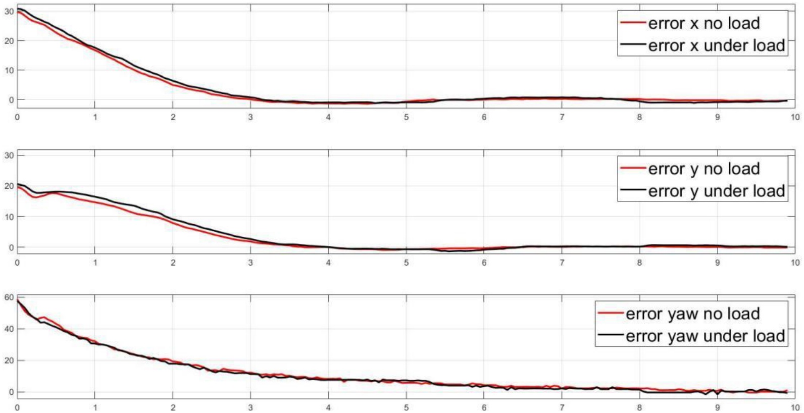
Figure 25.
Errors of robot with respect to target setpoint
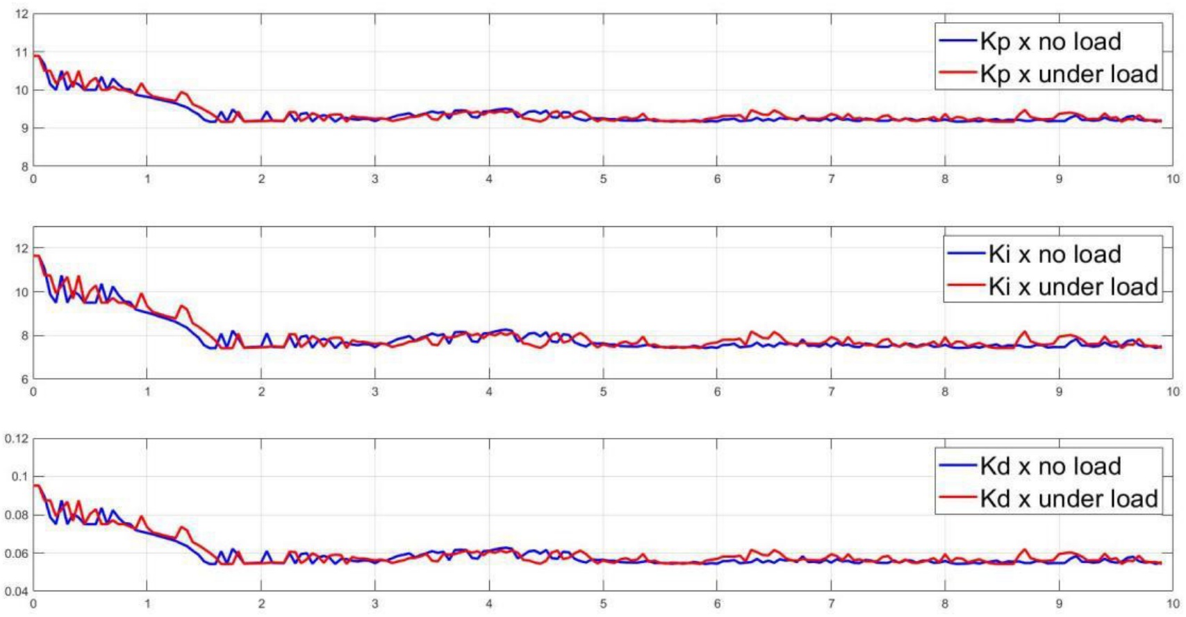
Figure 26.
PID Gains tuning results with respect target setpoint in x-dimension
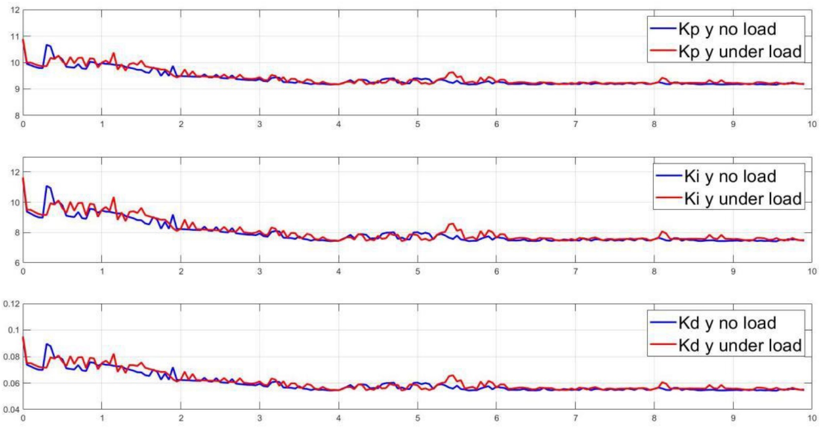
Figure 27.
PID Gains tuning results with respect to target setpoint y-dimension
5.2.2. Elliptical trajectory tracking control scenario
The designed controller is then put to the test to guide the robot in tracking an elliptical trajectory. The elliptical path is configured to be 50cm long and 30cm wide along the x-y directions, with a heading angle set at -45 degrees. The results of this control experiment are presented in Figure 28 through Figure 32. Figure 28 illustrates the tracking performance within the x-y plane, showcasing effective trajectory tracking with minimal error. Detailed control responses for the x, y positions, and yaw angle are depicted in Figure 30, demonstrating consistent performance comparable to the initial scenario. Additionally, the tuning results for the PID controllers are visualized in Figure 31 and Figure 32.
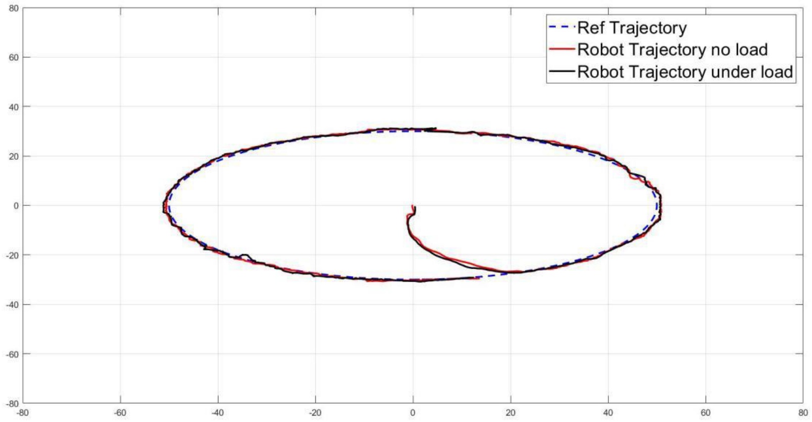
Figure 28.
Trajectory tracking responses with respect to elliptical trajectory in x-y plant
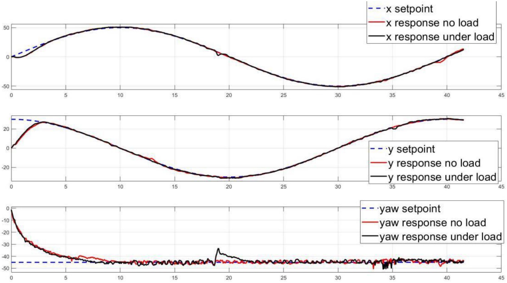
Figure 29.
Robot position responses with respect to elliptical trajectory
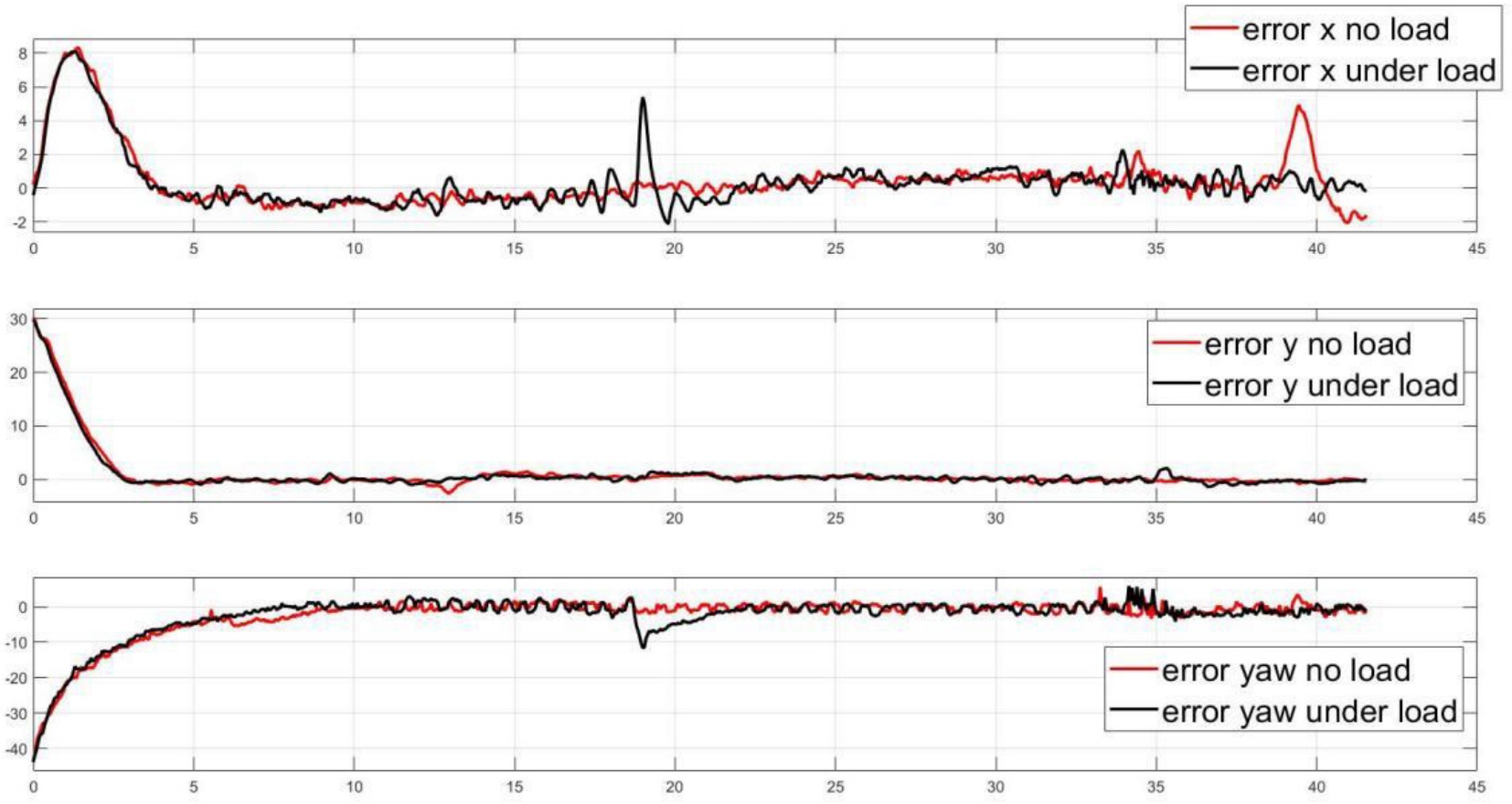
Figure 30.
Robot position tracking errors with respect to elliptical trajectory
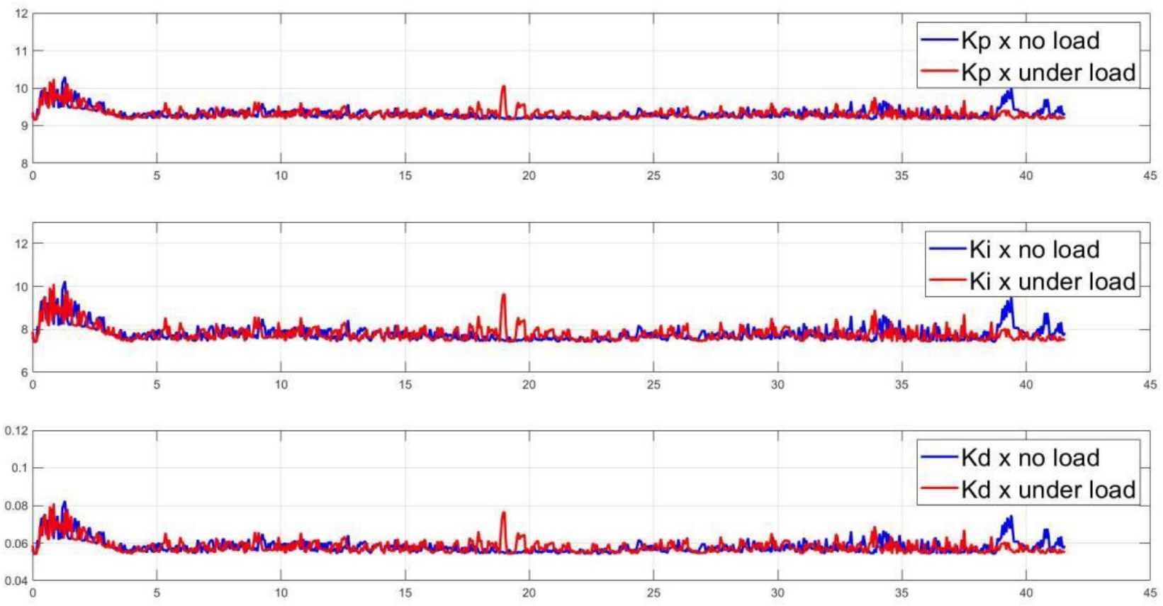
Figure 31.
PID gains tuning results with respect to elliptical trajectory in x dimension
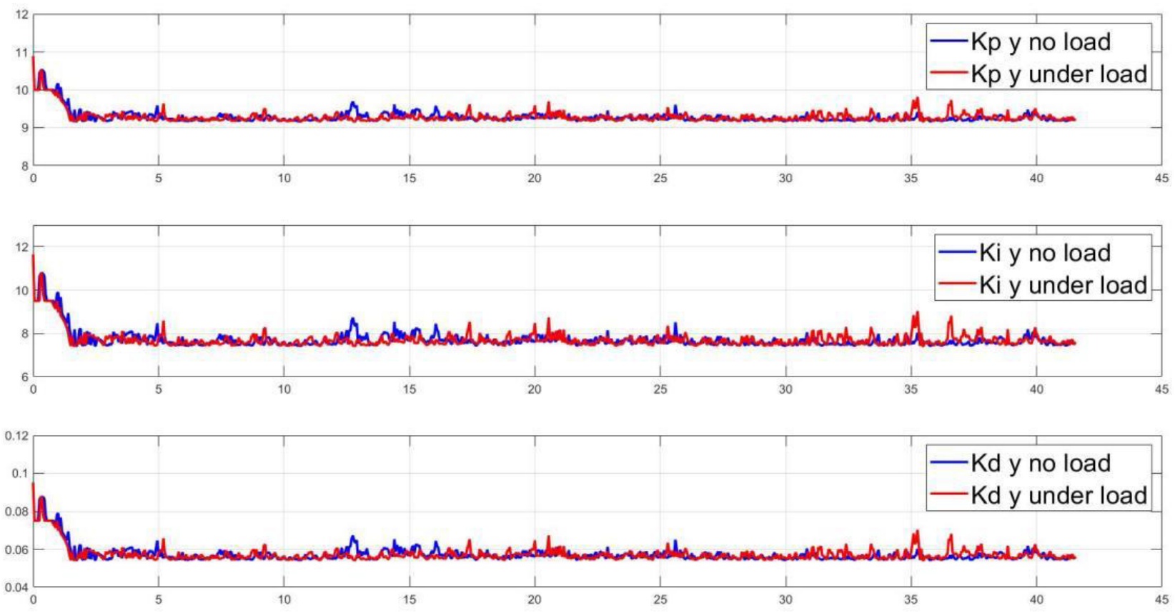
Figure 32.
PID gains tuning results with respect to elliptical trajectory in y dimension
5.2.3. Rectangular trajectory scenario
The final case examined under two loading conditions involves tracking a rectangular trajectory. In this experiment, the robot is configured to follow a rectangular path with dimensions of 80 cm in length along the x-direction and 60 cm in width along the y-direction, with a desired yaw angle set at 20 degrees. The control results are presented in Figure 33 rough Figure 35. These results demonstrate that the controller effectively guides the robot to track the desired trajectory, exhibiting minimal steady-state error and low overshoot. It’s notable that in this scenario, there is some overshoot due to sudden changes in the desired x-y direction, causing the robot, with its inertia, to continue moving in a certain direction.
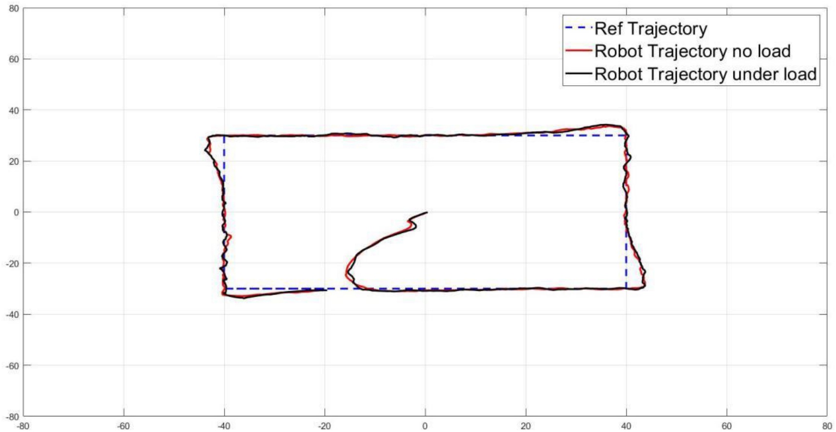
Figure 33.
Trajectory tracking responses with respect to rectangular trajectory in x-y plant
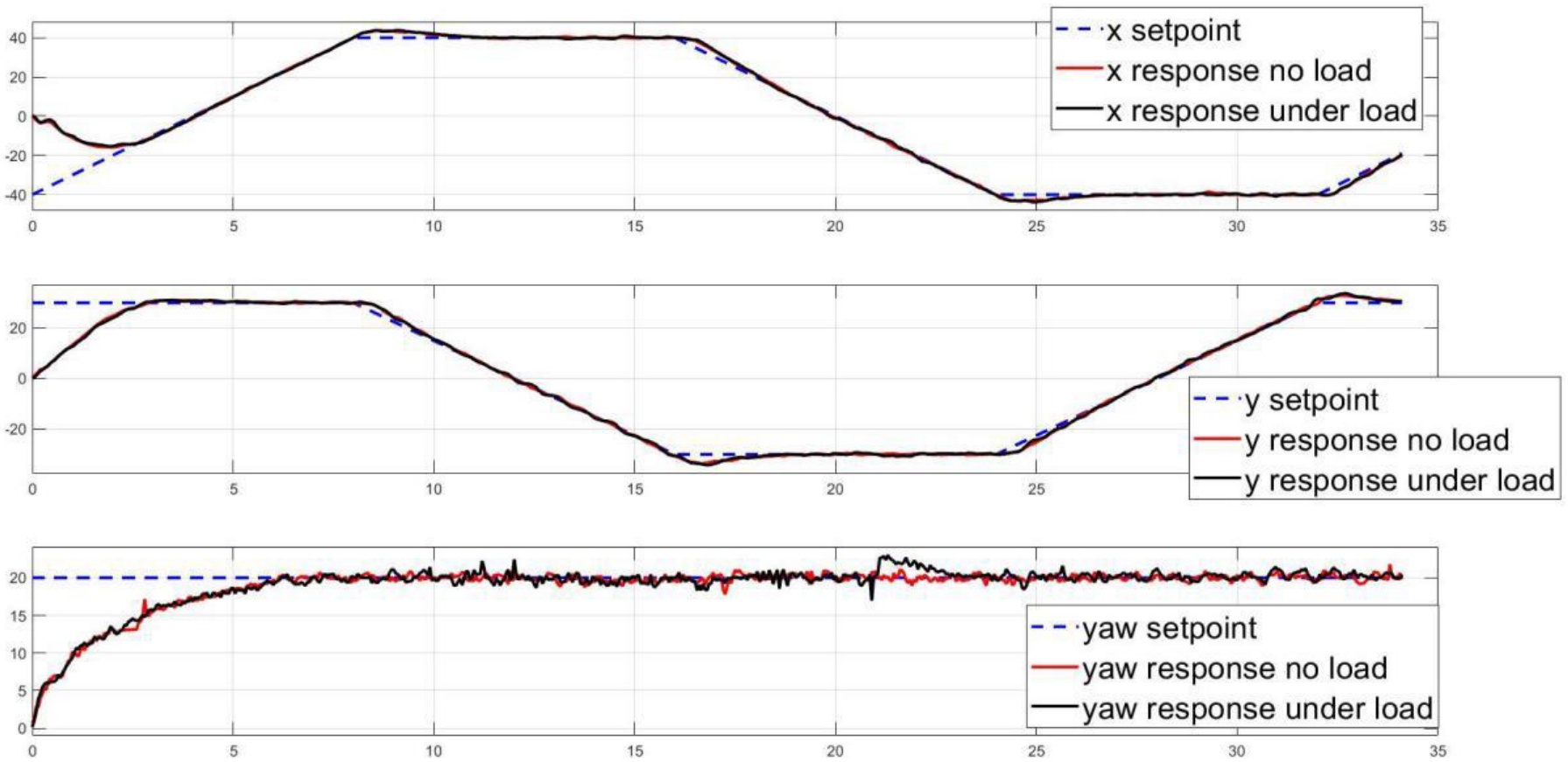
Figure 34.
Robot position responses with respect to rectangular trajectory
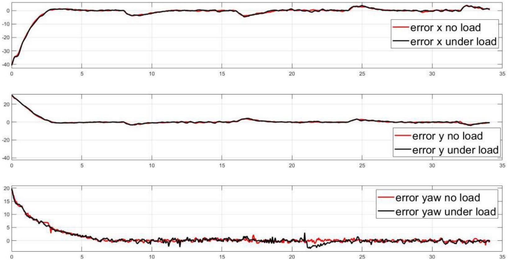
Figure 35.
Robot position tracking errors with respect to rectangular trajectory
In summary, to quantitatively assess the performance of the control system, the root mean square error (RMSE) values in the x, y, and yaw dimensions are calculated. Table 6 displays the RMSE values for different scenarios under both unload and load conditions. From the RMSE table, it is observed that the RMSE values for x and y dimensions in rectangular trajectory tracking are the largest, attributed to sudden changes in the desired trajectory. However, the RMSE values under load conditions do not show significant differences. This indicates that the designed controller effectively handles load conditions.
5.2.4. Circular trajectory and eight-shape trajectory scenarios
Moreover, the designed controller is evaluated for its ability to guide the robot along circular and eight-shaped trajectories. The control outcomes are illustrated in Figure 36 through Figure 41. Figure 36 to Figure 38 depict the tracking control results for the circular trajectory, while Figure 39 to Figure 41 display the results for the eight-shaped trajectory. Consistent with previous scenarios, the robot adeptly follows the circular path with commendable accuracy, maintaining a consistent shape throughout the trajectory. Overall, across various scenarios, the controller exhibits consistent performance and robustness, demonstrating its ability to adapt to different trajectories and load conditions.
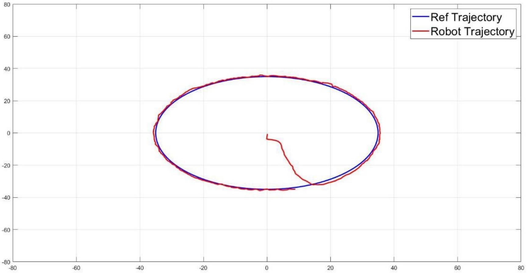
Figure 36.
Trajectory tracking response with respect to circular trajectory in x-y plant
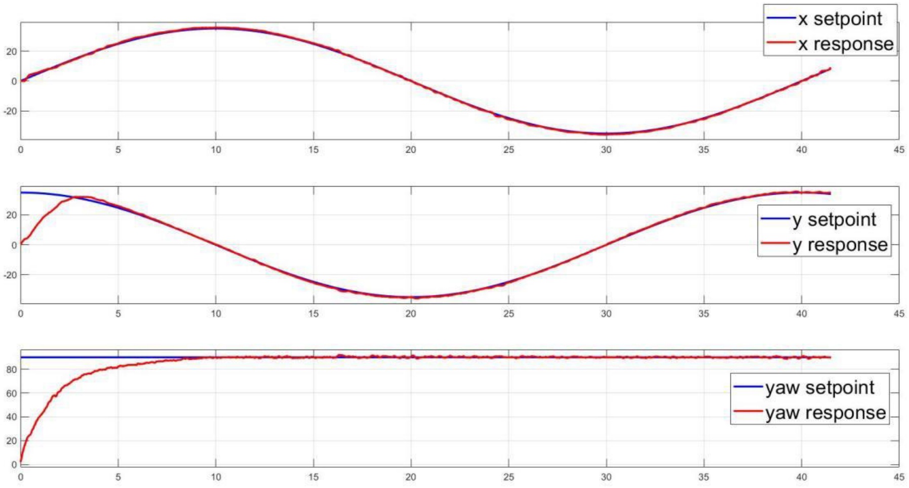
Figure 37.
x-y positions and yaw angle tracking control responses with respect to circular trajectory
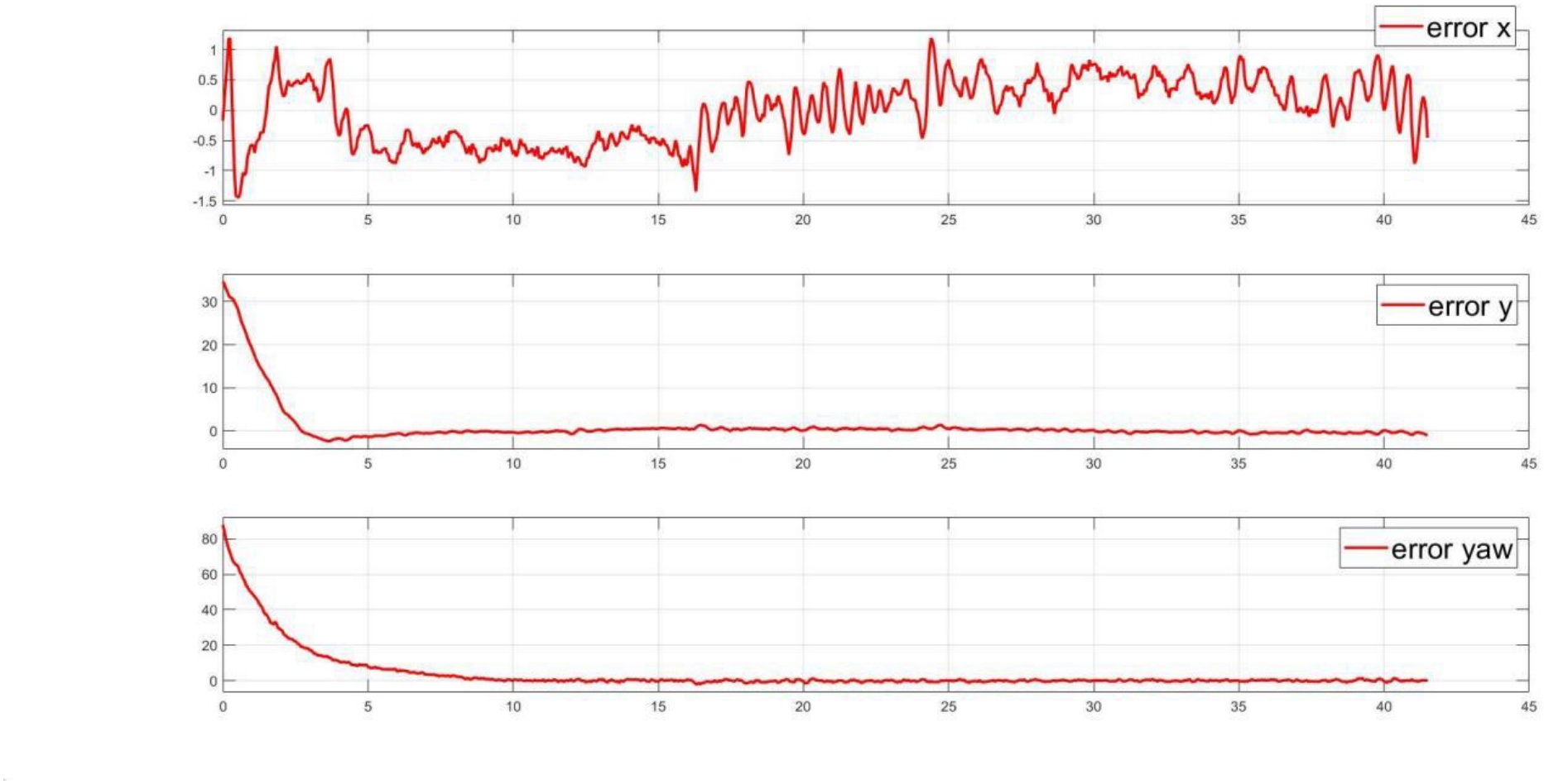
Figure 38.
Tracking errors with respect to circular trajectory
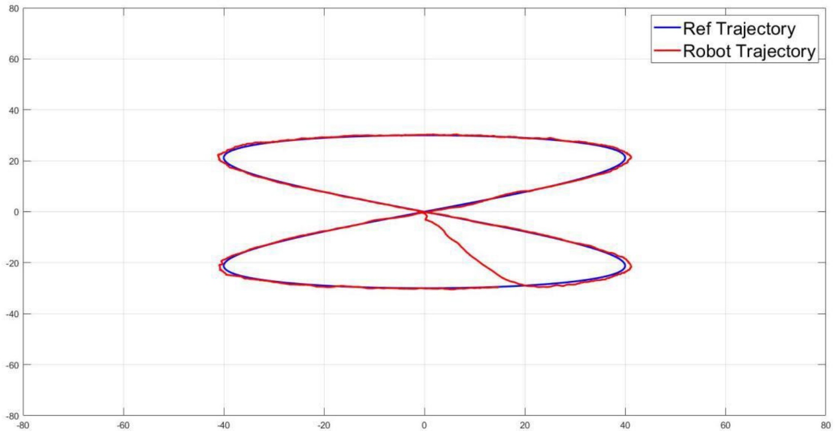
Figure 39.
Trajectory tracking response with respect to eight-shape trajectory in x-y plant
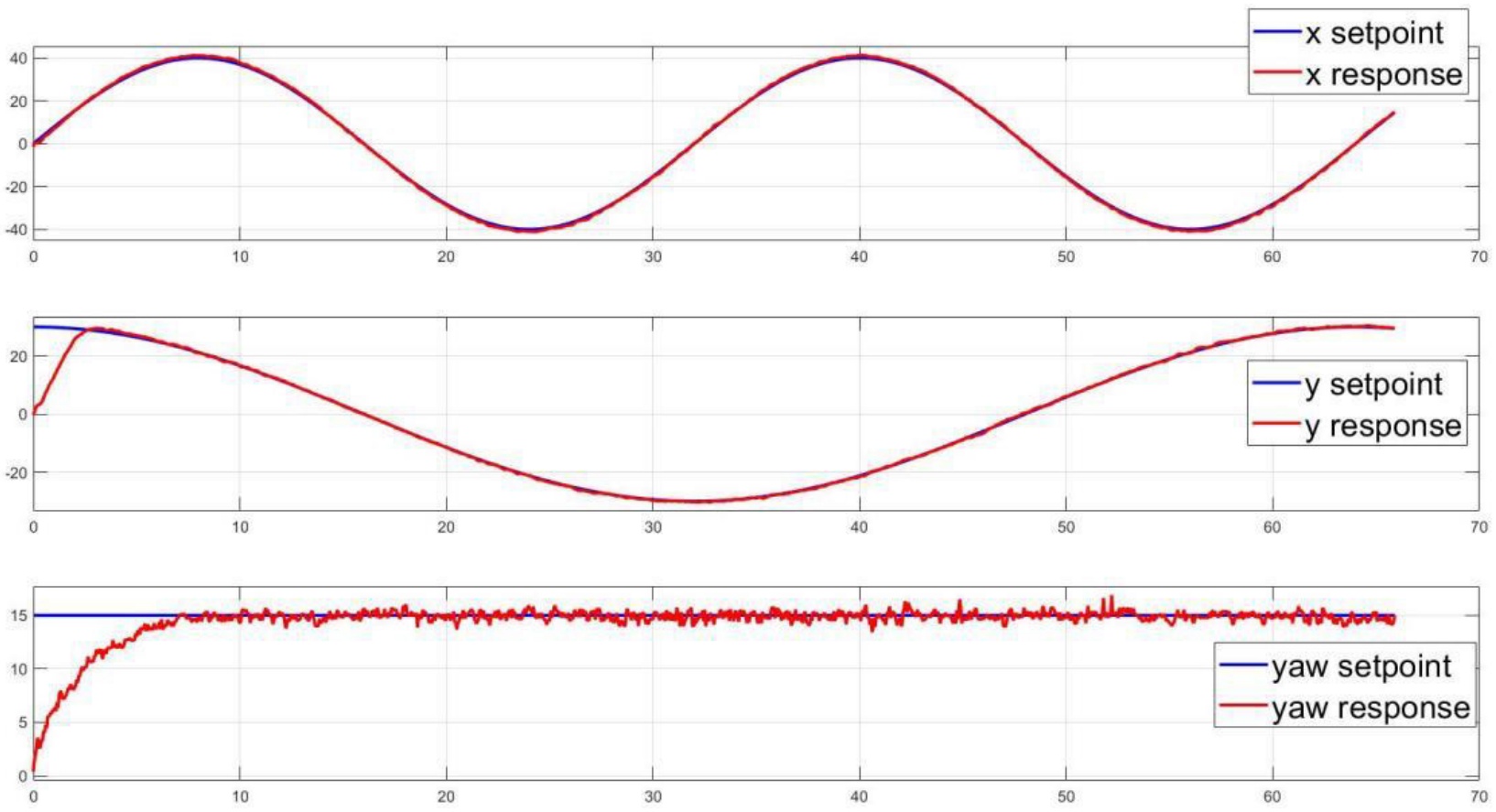
Figure 40.
x-y positions and yaw angle tracking control with respect to eight-shape trajectory
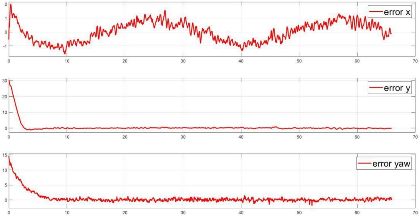
Figure 41.
Tracking errors with respect to eight-shape trajectory
5.3. Discussion
The accuracy and robustness of the Fuzzy-PID controller for four wheels mecanum robot trajectory tracking under numerous scenarios and loading conditions are shown by the simulation and experimental results reported in this paper. The results of the simulation demonstrate that when it comes to providing accurate and smooth tracking of complex trajectories, the fuzzy-PID controller outperforms the PID and fuzzy controllers. The ability of the Fuzzy-PID controller to combine the advantages of fuzzy logic with PID control accounts for its higher tracking accuracy when compared to the standalone Fuzzy and PID controllers.
The proposed control system’s performance in different trajectories, including desired position, elliptical, rectangular, circular, and eight-shaped path, is further validated by the experimental results. Excellent tracking precision, resilience, and adaptability are demonstrated by the control system in both loading conditions. Plots for trajectory tracking, response, error, and PID gain reveal the system’s capacity to maintain accurate tracking, stable performance, and smooth motion even when additional payloads are present.
A quantitative assessment of the tracking accuracy of the control system and the effect of the load on its operation is given by the RMSE analysis. The findings demonstrate that, despite a slight decrease in tracking accuracy brought about by the increased load, the control system is still able to maintain comparatively low RMSE values, guaranteeing accurate trajectory tracking and positional control. The load has varying effects on the different dimensions; the y-dimension is most affected, followed by the x- and yaw-dimensions. For mobile robots to be implemented in a variety of industrial and service sectors where payload weight frequently varies, the control system must be able to maintain consistent performance under changing load situations.
6. Conclusion
In this paper, a novel control approach of combining a Fuzzy-PID controller for position control and a Fuzzy controller for heading control has been proposed and investigated for the FMWMR. Moreover, a sensor fusion technique, which combines data from the camera and IMU, is also implemented for enhancing heading angle estimation. The control system’s outstanding performance in providing precise and smooth tracking of various trajectories under different loading cases has been proved by the results of simulations and experiments. Because of its versatility and resilience while managing changes in payload, the system has great promise for the real-world implementation of mobile robots in industrial and service applications. Our research’s finding advances the development of mobile robot control algorithms by leveraging the benefits provided by multi-sensor data fusion technique.
List of abbreviations
- FMWMR:
Four Mecanum-Wheeled Mobile Robots
- PID:
Proportional Integral Derivative
- GPS:
Global Positioning System
- IMU:
Inertial Measurement Unit
- COG:
Center Of Gravity
Declarations
[1] Availability of data and materials
The authors confirm that the data supporting the findings of this study are available within the article and its Supplementary material. Raw data that support findings of this study are available from the corresponding author, upon reasonable request.
[3] Financial disclosure Funding
This research is funded by Vietnam National University Ho Chi Minh City (VNU-HCM) under grant number C2021-20-15.
[4] Contributed by Authors’ contributions
Trong-Tai Nguyen conceived of the presented idea, developed the theory and performed the computations, prepared facilities for experimental, verified the analytical methods and results. Quang-Tho Le, Quang-Phuoc Pham, Tran-Long Le conducted experimental results. All authors discussed the results and contributed to the final manuscript.
ACKNOWLEDGEMENTS
We acknowledge the support of time and facilities from Ho Chi Minh City University of Technology (HCMUT), VNU-HCM for this study.