

1. Introduction
In process industries, where maintaining exact liquid levels in storage vessels is essential for product quality, safety, and effective operation, liquid level management is a basic [1,2,3]. Due to their structural strength and capacity to tolerate high internal pressures, spherical tanks are one of the most popular tank geometries [4, 5]. However, due to the nonlinear relationship between liquid volume and height, where the cross-sectional area varies with the square of the liquid height, spherical tank systems show notable nonlinear dynamics [6]. This significant nonlinearity poses a challenge to traditional control techniques, especially fixed-gain proportional-integral-derivative (PID) controllers, which frequently fail to provide adequate performance throughout the system’s whole operational range because of these fluctuating dynamics [7,8,9].
Because of its simplicity, ease of implementation, and shown performance in a variety of engineering applications, the PID controller continues to be the foundation of industrial-level control [10,11,12]. However, adjusting PID parameters for nonlinear systems like spherical tanks is difficult since traditional tuning techniques like Ziegler-Nichols or Cohen-Coon frequently result in less-than-ideal performance, particularly when there are considerable nonlinear behavior and outside disturbances [13, 14]. Furthermore, the performance of fixed-parameter PID controllers may degrade in terms of overshoot, settling time, and robustness against process uncertainty.
Metaheuristic optimization techniques have drawn a lot of interest in order to automatically tune PID gains by minimizing specified performance parameters (such as ITAE, ISE, IAE, overshoot, and energy consumption) in order to meet these tuning difficulties [15,16,17]. Among these, two widely researched nature inspired methods are Whale Optimization Algorithm (WOA) and Genetic Algorithms (GA). While WOA mimics the bubble-net hunting method of humpback whales, exhibiting significant global search capabilities, GA mimics evolutionary selection and genetic operations to effectively traverse search spaces [18]. By combining both strategies, PID parameters in challenging nonlinear control systems can be optimized more successfully by utilizing the resilience of GA and the balance between exploration and exploitation of WOA.
The efficiency of hybrid and enhanced metaheuristic algorithms in fine-tuning PID and sophisticated controllers for nonlinear systems has been demonstrated in recent studies. In comparison to traditional tuning techniques, hybrid metaheuristic algorithms have been used for optimal PID tuning in a variety of domains, resulting in better set-point tracking and disturbance rejection. Furthermore, research on spherical tank control indicates that closed-loop performance may be greatly enhanced over traditional controllers by model-based and optimization-driven tuning.
Despite these developments, there remains a dearth of research on hybrid WOA-GA optimization for spherical-tank PID level control. This serves as the driving force behind the current study, which develops a hybrid WOA-GA method to adjust PID settings for a nonlinear spherical tank system. By reducing performance metrics like integrated time-absolute error (ITAE), overshoot, and settling time, the suggested approach seeks to provide reliable and ideal control across the operating range [19]. The hybrid WOA-GA tuned PID controller outperforms single optimization algorithm techniques and traditional tuning methods, according to simulation and real-time experimentation findings. The primary contributions include:
- Obtaining the mathematical model of a nonlinear spherical tank system. The complete operating region of the tank is taken into account while modeling.
- The obtained model is a second-order type, capturing the inherent nonlinear dynamics of the plant and its impact on level control.
- Design and deployment of control strategies like GA-PID, WOA-PID, and proposed control strategies, hybrid WOAGA-PID for controlling the level in a spherical tank.
- The performance of the control strategies are evaluated through simulations and real-time deployments, such as variations in reference values, disturbances and robustness.
- The performance of control strategies are evaluated based on their transient responses and performance metrics such as ISE, IAE and ITAE, and control effoers providing a comprehensive analysis of their effectiveness.
The rest of the paper is organized as follows: Section 2 describes the mathematical modeling of the process. Section 3 discusses the design of various controllers used in the system as well as controllers used for comparison. Section 4 describes the simulation and real-time results discussion. Finally, the paper concludes in Section 5.
2. Modeling of System
System model identification of a nonlinear spherical tank involves deriving a mathematical representation that captures the tank’s dynamic behavior. Due to the construction geometry, the relationship between the inlet flow rate and liquid level is not linear. Accurate modeling typically requires experimental data and techniques like system identification. A spherical tank of radius R containing an incompressible liquid. Let the liquid level at time t be h(t). The inlet flow rate is denoted by fin(t) and the outlet flow rate by fout(t). Figure 1 shows the schematic of spherical tank system. The fundamental mass balance for the tank is given by,
where V is the volume of liquid in the tank. For a spherical tank of radius R, the volume of liquid up to height h is expressed as, The cross-sectional area of the tank at height h is obtained by differentiating the volume with respect to h: Using the chain rule, Substituting this into the mass balance equation gives Hence, the nonlinear dynamic model of the spherical tank is The outlet flow is governed by gravity through a valve and it is given by, where Cd is the discharge coefficient, and g is the acceleration due to gravity. Substituting equation (7) into the dynamic equation (6) yields, At steady state, the liquid level remains constant, and therefore which leads to where hs denotes the steady-state liquid level. The inlet flow is manipulated through a pump whose dynamics can be approximated by a first-order system: where Ka is the actuator gain and τa is the actuator time constant. The overall transfer function from the control input U(s) to the liquid level H(s) is obtained by cascading the actuator and the process models: Thus, the second-order transfer function of the spherical tank level system is Expanding the denominator, the transfer function can be written in standard second-order form as, where The spherical tank alone exhibits first-order dynamics. The inclusion of actuator dynamics results in a second-order transfer function, which more accurately represents the practical system behavior and is commonly used for controller design and analysis.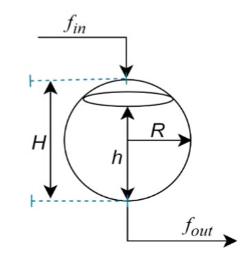
Figure 1.
Schematic of a spherical tank
2.1. Laboratory Setup of Spherical Tank System
The laboratory setup of the system consists of a spherical tank, pump, variable frequency drive (VFD), hydrostatic pressure transmitter, reservoir tank, manual inlet/outlet control valve, interfacing module, and personal computer (PC) as shown in Figures 2 and 3. The hydrostatic pressure transmitter acts as a feedback measurement device to measure the liquid level in the tank, and it converts the level into a 4-20 mA signal. The output is interfaced through the NI DQA 6001 card to the computer using a USB, where it converts it into a voltage in the range of 1-6 volts. The control program was written in Simulink using MATLAB 2013b software. Based on the controller’s gain and the VFD’s frequency, the error signal proceeds to initiate instantaneous control action that creates the necessary water flow in a tank. Figure 2 depicts the spherical tank’s real-time experimental setup with the regulated level. The specifications for the real-time process requirements are listed in Table 1 and are shown below: The System Identification Toolbox in MATLAB provides a comprehensive set of tools for developing dynamic system models using measured input–output data. The procedure usually starts with collecting appropriate input and output signals that capture the system’s behavior under different operating conditions. After data collection, the next step involves preprocessing to eliminate noise, outliers, and unwanted trends that could interfere with accurate system identification. Once the data are refined, an appropriate model structure such as a second-order transfer function is chosen based on existing system knowledge or exploratory data analysis.
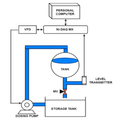
Figure 2.
Block diagram of level setup
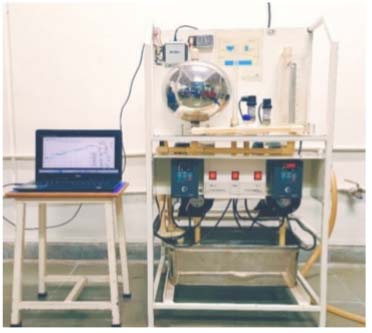
Figure 3.
Schematic of interfacing of NI DQA USB 6001 module with spherical tank system
Table 1.
Technical specification of experimental setup
| Sr.No | Components | Specification |
|---|---|---|
| 1 | Spherical Tank | SS, H-25 cm, D-25cm, R-12.5 cm |
| 2 | DAQ Device | NI USB6001, 14 bit, AI-4, AO-2 |
| 3 | Level Transmitter | Two wires, Range 0-250mm, O/P=4 to 20 mA |
| 4 | Dosing Pump | PDDP with adjustable stroke |
| 5 | VFD | 1-ph 200 VAC, 1.1 A, O/P AC 3-ph, 0-230v |
| 6 | Manual outlet valve | Cd = 19.69 cm2/s |
| 7 | Input flow rate | fin = 0 (Min) and 420 (Max) LPH |
| 8 | Output flow rate | fout = It is kept 150 LPH for study |
The MATLAB System Identification Toolbox then applies estimation algorithms, such as least-squares and prediction error minimization methods, to determine the optimal parameters for the selected model.
The model’s accuracy is assessed through validation techniques, typically by comparing its predicted output with a separate set of measured data. If the results are unsatisfactory, the process can be repeated by modifying the model structure, estimation method, or preprocessing approach. The final identified transfer function can then be utilized for system analysis, controller design, and simulation tasks.
Identifying accurate transfer functions is essential in many engineering fields, as it provides a mathematical model that captures the dynamic characteristics of a system. Such models are vital for designing robust control strategies, forecasting system behavior, and enhancing overall system performance. Figure 4 illustrates the model identification and validation results. The y-axis represents the liquid level in terms of a voltage signal, ranging from 1 V to 6 V, corresponding to a tank liquid level of 0 cm to 22 cm.
The system identification process produced a second-order transfer function model that achieved a 94.81% fit with the estimation data. The resulting transfer function is expressed as follows:
This mathematical model (16) is used to design the PID controller.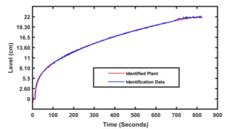
Figure 4.
Open loop response of spherical tank
3. Controller Design
This section covers the design and tuning of various controllers, including GA-PID, WOA-PID, and WOAGA-PID controllers. The tuning techniques aim to enhance system stability and performance. A comparison of these methods is provided to evaluate their effectiveness. The analysis includes key performance metrics such as settling time, overshoot, and steady-state error.
3.1. General PID Controller Structure
PID controllers should be configured to a level where there are no faults between process variables and set points to ensure rapid response. When the system’s parameters change or are unknown, the PID controller’s capabilities are constrained. Because of its low cost, it is utilized in industrial processes most frequently. The general control structure of the PID controller is given in Figure 5. Many nonlinear processes are controlled with an industrially proven PID controller. A PID controller may manage several intricate and nonlinear processes and offers physical tweaking. Equation 17 represents the commonly used structure of PID controller.
In this representation, the proportional gain is kp = kc, the integral time is Ti and ki = kc/Ti and e(t) is the error value.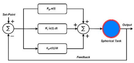
Figure 5.
Structure of PID controller
3.2. Whale Optimization Algorithm
The Whale Optimization Algorithm is a metaheuristic optimization algorithm inspired by humpback whales’ distinctive hunting tactic, bubble-net feeding [20, 21]. This sophisticated foraging behavior involves whales creating distinctive bubble formations to encircle and disorient their prey, primarily krill and small fish, before moving towards the concentrated food source [22, 23]. The algorithm emulates this hunting technique through a series of mathematical models that represent the key phases of the bubble-net feeding process, offering a novel approach to solving complex optimization problems across various domains. The Whale Optimization Algorithm’s mathematical formulation is based on the modeling of three primary behaviors: seeking for prey, bubble-net attacking, and encircling prey [24]. As shown in equation 18, an ITAE is employed as the fitness function,
Enclosing Prey: The WOA implies that the target prey is the current best-to-date solution since the prey in the search space is unknown. The other whale will then attempt to reposition themselves in relation to the intended victim. When |X| > 1, whales search globally instead of attacking.
Distance calculation
Position update
where, X, Y=Vectors which controls exploration and exploitation. W(t)=Current position of whale, Wrand(t) Best solution (Position of Prey). and t is current iteration where, X and Y are coefficient vectors, α decreases linearly from 2 to 0 and (rand) is random vector in [0,1]. The selection of this operator depends on the coefficient vector X and a random number rand, where rand is a random number in [0, 1]. For each individual, if rand < 0.5 and |X| < 1, the position is updated by encircling prey.Attacking Phase: If rand > 0.5, the bubble-net predation stage begins. The mathematical model of the search is as follows.
Where, L′=|Wrand(t) − W(t)|, ‘l’ is a random value between -1 and 1, ‘c’ is the constant which denotes the shape of the logarithmic spiral.Searching for Prey: If rand < 0.5 and |X| ≥ 1, the individuals need to expand their exploration areas. This phase uses a randomly generated set of solutions Wrand(t) to update the individuals’ locations, which allows the WOA algorithm to perform a global search. The rules of the update solution are as follows.
3.3. Genetic Algorithm
The GA is a random global search and optimization technique that was created by mimicking the natural biological evolution process. During the search process, it may automatically gather information about the search space, and adaptively manage the search procedure to find the optimal answer. Every member of the population is a potential solution to the optimization issue. The fitness function evaluates an individual’s capacity for adaptability. Those with high levels of fitness are able to procreate while those with low levels of fitness are removed. To create a new population during reproduction, selection, crossover, and variation are required. Finally, a better answer will be found [25].
3.4. Hybrid WOA-GA Algorithm
Figure 6 depicts the flowchart of the proposed WOA-GA method, and Figure 7 shows the block diagram of WOAGA-PID controller.
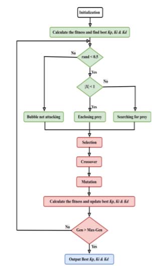
Figure 6.
WOA-GA algorithm process flowchart
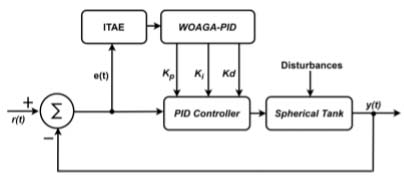
Figure 7.
Block diagram of proposed WOA-GA based PID controller
Step 1: Establish the starting settings, including Popsize, MaxGen, lower bound, upper bound, and number of variables. Next, a starting population is chosen at random.
Step 2: Calculate the fitness value of each individual using Equation (18) and find best solution Kp, Ki, Kd.
Step 3: Update the populations by WOA. If rand < 0.5 and |X| < 1, individuals are updated by encircling prey using Equations (19)–(20). If rand < 0.5 and |X| ≥ 1, individuals are updated by searching for prey using Equation (22). If rand > 0.5, individuals are updated by bubble-net attacking using Equation (21).
Step 4: Use GA to update the population the related operators make use of mutation, crossover, and the roulette wheel selection approach.
Step 5: Calculate the fitness value of each individual and update best solution Kp, Ki, Kd.
Step 6: If t < MaxGen, then t = t + 1, update a, X, Y, c, l and rand, and return to step 3. If t = MaxGen, then the best fitness and global-best Kp, Ki, Kd are obtained. The main optimization parameters for GA, WOA, and the hybrid WOA–GA, such as limits, population size, and number of generations, are compiled in the Table 2. Crossover and mutation for GA and the control parameter α dropping from 2 to 0 for WOA and WOA–GA are highlighted. The Table 3 displays differences in Kp, Ki, and Kd resulting from various search strategies and compares PID controller gains acquired using GA, WOA, and hybrid WOA–GA optimization.
Table 2.
Optimization Parameters
| Parameter | GA | WOA | WOA-GA |
|---|---|---|---|
| Lower bound [Kp, Ki, Kd] | [1, 0.01, -20] | [1, 0.01, -20] | [1, 0.01, -20] |
| Upper bound [Kp, Ki, Kd] | [5, 3, 5] | [5, 3, 5] | [5, 3, 5] |
| No. of Generations | 20.0 | 20.0 | 20.0 |
| No. of Population | 20.0 | 20.0 | 20.0 |
| Crossover Fraction | 0.8 | – | 0.8 |
| Mutation Fraction | 0.2 | – | 0.2 |
| α decrease | – | 2 to 0 | 2 to 0 |
Table 3.
Controller tuning values
| Sr.No. | Controller Type | Kp | Ki | Kd |
|---|---|---|---|---|
| 1 | GA-PID | 1.15 | 0.03 | -34.34 |
| 2 | WOA-PID | 2.56 | 0.17 | 1.31 |
| 3 | WOA-GA-PID | 1.92 | 0.2 | -7.27 |
The optimizer discovered a derivative action that mitigates to counteract excessive damping introduced by the plant as indicated by the negative Kd in GA-PID.
Figure 8 compares the convergence characteristic curve of level control of spherical tank obtained by GA, WOA and WOAGA for a population size of 20. The convergence curves confirm that the control method presented based on GA, WOA and WOAGA reaches a sensible degree of performance in controlling level. It is clearly noticeable that WOAGA converges to a small error, compared to GA and WOA.
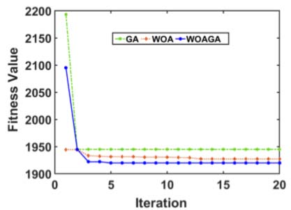
Figure 8.
Convergence curves of GA, WOA and WOAGA with population size 20
4. Results and Discussion
This section presents the simulation and real-time results of liquid level control in a spherical tank considering its nonlinear mathematical model. The performance of each control strategy was verified through simulation and real-time for different scenarios where the control variable was affected. For a quantitative assessment of the results of each controller in terms of response quality and error value, which allows for comparing them with one another, several Performance Indices were calculated. A MATLAB R2023b/SIMULINK software is used in simulation and real-time analysis to evaluate the output performance of the liquid level of a spherical tank under various controller configurations. The tank’s liquid level range (0–22 cm) is used to control each region’s level.
4.1. Simulation Results
The performance of the designed controllers are tested to regulate the liquid level in a spherical tank. All controllers are designed using the obtained mathematical model of the spherical tank. The desired set values of the level is 19.30 cm, and the simulation is run for 1000 seconds. The closed-loop responses for the designed controllers are shown in Figure 9 (a) and (b) depict the simulation output responses and control efforts taken by all designed controllers, respectively. The response of the controllers are recorded in terms of rise time, peak time, settling time, and overshoot percentage, also the performance indices ISE, IAE, and ITAE are captured, which are shown in Tables 4 and 5, respectively. Table 4 allows for a more precise analysis of the behavior of the control strategies by verifying their transient response. The simulation results demonstrate that the WOAGA optimized PID controller outperforms other tuning methods, achieving the shortest rise time of 193 seconds, the fastest peak time 302 seconds, minimal overshoot of 1.25%, and fastest settling time of 251 seconds. While GA-PID and WOA-PID exhibit comparable rise times of 254 and 237 seconds, respectively, WOAGA-PID’s superior dynamic response highlights its effectiveness in balancing speed and stability. Notably, GA-PID suffers from excessive overshoot of 3.21%, emphasizing challenges in conventional tuning for complex systems.
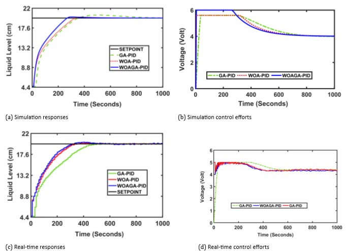
Figure 9.
Simulation and real-time control efforts and responses
Table 4.
Time domain comparison between simulation and real-time implementation
| Set Point | Specification | Simulation | Real-Time | ||||
|---|---|---|---|---|---|---|---|
| GA-PID | WOA-PID | WOAGA-PID | GA-PID | WOA-PID | WOAGA-PID | ||
| 19.30 cm Level | Rise Time | 254 | 237 | 193 | 305 | 275 | 210 |
| Peak Time | 504 | 374 | 302 | 512 | 398 | 347 | |
| Settling Time | 670 | 307 | 251 | 680 | 325 | 274 | |
| Overshoot % | 3.21 | 1.04 | 1.25 | 2.78 | 1.56 | 1.67 | |
Table 5.
Comparison of performance parameters in simulation and real-time implementation
| Set Point | Controller | Simulation | Real-Time | ||||
|---|---|---|---|---|---|---|---|
| ISE | IAE | ITAE | ISE | IAE | ITAE | ||
| 19.30 cm Level | GA-PID | 624 | 462 | 7004 | 648 | 492 | 8422 |
| WOA-PID | 614 | 361 | 3732 | 657 | 412 | 4757 | |
| WOAGA-PID | 518 | 300 | 2604 | 638 | 398 | 3228 | |
WOAGA-based methods consistently reduce overshoot compared to GA and slitely more than WOA approaches, validating their robustness in optimizing control performance across multiple time-domain criteria. Table 5 reports the performance indices calculated for this scenario in a time of 1000 seconds. The novel WOAGA-optimized PID controller achieves the lowest ISE (518), IAE (300), and ITAE (2604), confirming its superior error minimization and transient response compared to GA-PID and WOA-PID methods.
It is also observed WOAGA-PID also outperforms than GA-PID and WOA-PID controllers in IAE and ITAE, emphasizing WOAGA desiged PID efficacy in reducing cumulative errors. GA-PID exhibits the poorest performance ITAE (7004), likely due to oscillatory behavior, while WOA-PID shows balanced but suboptimal metrics.
These results reinforce WOAGA-optimized controllers as robust solutions for precision and stability in level control systems. The Figure 10 depicts the setpoint tracking performance of all designed controllers and observed that WOAGA-PID outperforming than GA-PID and WOA-PID. GA-PID response is sluggish to achieve the changed setpoint. This comparison shows that the WOAGA-PID controllers superior robustness.
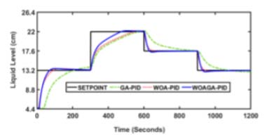
Figure 10.
Setpoint tracking
4.2. Real-time implementation results
To prove the efficacy of designed controllers, the simulation results are validated through real-time implementation on a laboratory set-up of a nonlinear spherical tank system. The closed loop performance of the designed GA-PID, WOA-PID, and hybrid WOAGA optimized-PID controllers are presented to support the claim. Figure 9 (c) and (d) depicts the real-time responses and their control efforts for reference tracking performance for the setpoint of 19.30 cm level, respectively. From this it’s observed that the WOAGA-PID controller is performing best among the rest of the controllers. The hybrid WOAGA-PID controller shows better performance in a real-time environment, achieving the fastest rise time of 210 seconds, the lowest settling time of 274 seconds, and minimal overshoot of 1.67% as given in Table 4, while giving optimal error metrics (ISE: 638, IAE: 398, ITAE: 3228), outperforming all counterparts. WOA-PID shows moderate overshoot 1.56% and reduced ITAE (4757) compared to GA-PID (ITAE: 8422) reported in Table 5. Notably, WOAGA-PID’s balanced performance combining rapid response, stability, and precision validates WOAGA adaptability to real world disturbances. While WOAGA and WOA methods exhibit trade-offs GA-PID’s high sluggishness, WOAGA optimized control consistently bridges speed and accuracy, proving its robustness in practical implementations. from analysis it is observed that the values recoded in real time are slightly more than simulation, because of inherent hardware limitations and dynamics. Another hardware limitation is that it does not work for control signals more than six volts. Its working range is one to six volts, which converts it into 0 to 50 Hz to control the speed of the pump. Based on the data in Table 6, the hybrid WOAGA-PID controller consistently exhibits the lowest control effort in both simulation and real-time implementation, indicating improved energy efficiency compared to GA-PID and WOA-PID controllers. Moreover, the reduced norms in real-time operation demonstrate the robustness and practical effectiveness of the proposed hybrid approach under experimental conditions. The WOAGA-PID controller demonstrates superior disturbance rejection by exhibiting the smallest deviation from the setpoint and the fastest recovery following the disturbance. In contrast, GA-PID and WOA-PID show larger transient dips and slower settling, indicating reduced robustness under disturbance conditions as depicted in Figure 11.
Table 6.
Comparison of control effort in simulation and real-time
| Norm | Simulation | Real-Time | ||||
|---|---|---|---|---|---|---|
| GA-PID | WOA-PID | WOAGA-PID | GA-PID | WOA-PID | WOAGA-PID | |
| norm 2 | 143.79 | 141.34 | 139.51 | 145.18 | 143.71 | 142 |
| norm ∞ | 6 | 5.6 | 5.6 | 5.7 | 5.7 | 5.2 |
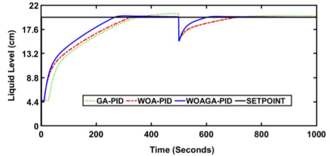
Figure 11.
Disturbnce rejection
5. Conclusion
This paper presents the successful design and implementation of an optimal PID level control strategy for a nonlinear spherical tank system using a hybrid WOA–GA. The proposed hybrid approach effectively combines the fast exploitation capability of WOA with the global search strength of GA to achieve reliable PID tuning for nonlinear process dynamics. Comparative simulation studies demonstrate that the WOAGA–PID controller outperforms WOA–PID and GA–PID controllers in terms of transient response, robustness, and standard performance indices. The effectiveness of the proposed method is further confirmed through real-time experimental validation on a laboratory-scale spherical tank, showing excellent set-point tracking and disturbance rejection under varying operating conditions. Overall, the results establish the proposed hybrid WOA–GA–based PID controller as an effective and practical solution for nonlinear level control applications, with strong potential for extension to other complex industrial processes. Future research will extend this approach to adaptive or predictive control frameworks with comprehensive uncertainty, noise, and large-scale experimental validation.