

1. Introduction
Inductive components play a crucial role in power conversion devices [1], telecommunications [2], and the automotive industry [3]. However, despite the fact that the total yearly turnover of the inductive components market exceeds 23 billion US$ [4], its operational parameters selection process is often based on a set of rules of thumb, common practices, and rough estimations. The primary barrier to the efficient optimization process of inductive components is the limited applicability of the components commonly used physical models. These physical models primarily rely on the linearization of characteristics or are restricted to a narrow range of operating parameters.
The gyrator-capacitor model presents an opportunity to overcome this limited applicability problem, enabling the efficient modeling of inductive component characteristics in the SPICE (Simulation Program with Integrated Circuit Emphasis) environment [5]. However, from the perspective of the power conversion device and automotive industries, the most important thing is accurately modeling the power loss characteristics of the inductive component. From the physical point of view, inductive component power losses consist of hysteresis losses, eddy current losses, and excess (also known as anomalous) losses [6, 7]. In the case of power conversion devices operating at driving frequencies up to 50 kHz, eddy current losses play a key role in efficient modeling. While there is a large variety of eddy current loss models [8, 9, 10, 11, 12], the commonly used gyrator-capacitor model utilizes the approach presented by Bertotti et al. [13]. This approach simplifies the model through a constant-value resistor that describes eddy current losses. However, the proposed approach of eddy current losses in the gyrator-capacitor model of the inductive component for SPICE modeling has not yet been directly validated.
This article fills this gap. The eddy current losses of a ring-shaped core made of nanocrystalline alloy were measured directly using an advanced hysteresis graph in the frequency range direct current to 36 kHz. In this frequency range, eddy current losses are the primary power losses in the inductive component. Next, the gyrator-capacitor model was implemented in the LTspice environment [14] offered by Linear Technology. Finally, the modeling results were compared with experimental measurements, enabling validation of the eddy current-based loss model for inductive components.
2. The material and methods of experimental investigation
A commercially available Vacuumschmeltze W915 core was used for the experimental investigation. It is a core made of nanocrystalline material, Vitroperm 500F, with the following chemical composition: Fe73.5Cu1Nb3Si15.5B7. The core was a ribbon-wound ring core in the form of a toroid, with magnetic material dimensions of 6.5 mm × 9.8 mm × 4.5 mm (inner diameter, outer diameter, height). The sample was deliberately selected to be as small as possible, so that the induced voltage in the flux density (B) induction measurements was as low as possible and within the measuring range of the hysteresis graph. Hysteresis loop measurements were performed using an AMH-200K-S device (Laboratorio Elettrofisico, Milan, Italy). The samples were magnetized with sinusoidal excitation, with an amplitude of 350 A/m, and the magnetization frequency (f) ranged from 1 to 36 kHz. Due to its high permeability, the sample was magnetized using only two turns of the coil, wound symmetrically on the sample. Figure 1 presents the results of the hysteresis loop measurements as a function of frequency.
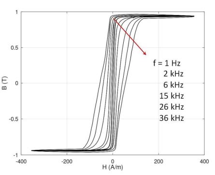
Figure 1.
Results of experimental measurements of the B(H) hysteresis loop as a function of magnetizing field frequency (f) for the Fe73.5Cu1Nb3Si15.5B7 (Vitroperm 500F) nanocrystalline alloy. Consecutive values of frequency follow the direction indicated by the arrow
3. Method of modeling
The proposed model of a nonlinear magnetic core was implemented in LTspice [14]. The gyrator circuit [15] with a gyrator resistance of 1/N [16] was enhanced by incorporating two ultra-high-value resistors to improve the circuit’s numerical stability. From a technical point of view, in this case, N should be considered the number of winding turns on the modeled magnetic core.
In the gyrator-capacitor method of modeling [17], the anhysteretic magnetization curve Bah(H) is modeled by the nonlinear variable capacitor C1. Next, the hysteretic losses (caused by the eddy currents) are added by the resistor (R3). The simplified schematic diagram of the gyrator-capacitor circuit for modeling an inductor with the nonlinear magnetic core is presented in Figure 2.
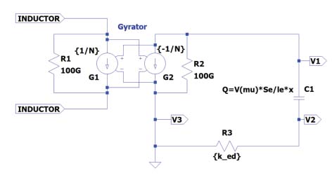
Figure 2.
The gyrator-capacitor circuit for modeling an inductor with the magnetic core exhibits nonlinear magnetization characteristics
The nonlinear relative magnetic characteristic can be modeled by the nonlinear capacitor C1. In such a case [18, 19]:
Se is the core’s cross-section, le is the length of the magnetic circuit of the core, and μ0 is the magnetic constant. In the LTspice software, the nonlinear capacitor is modeled considering its charge Q [18] in the following form:
In Equation 2, x is a voltage at capacitor, V(μr ∙ μ0) is the tabularized form of μr(H)∙μ0 provided to the simulation as a separate nonlinear voltage source, and x is the voltage at the nonlinear capacitor C1 [18]. Presenting nonlinear capacitors in this form in the LTspice model enables stable and efficient solutions to differential equations describing the state of the nonlinear system.
The proposed model neglects two additional sources of power losses in the core: static hysteresis losses and excess losses [18]. Although such losses can be replicated in the gyrator-capacitor model [18, 20], in the case of the nanocrystalline ribbon ring core (such as the Vacuumschmeltze W915 made of Fe73.5Cu1Nb3Si15.5B7 alloy), the static hysteresis loop B(H) has an area of about two orders of magnitude smaller than the area of the loop measured at a frequency of 36 kHz. As a result, the static hysteresis is neglected without significantly influencing the model’s accuracy, and an anhysteretic loop represents the nonlinear part of the magnetization curve.
The value of excess losses is directly connected to the value of saturation magnetostriction (λs) of anisotropic alloy [21]. The Fe73.5Cu1Nb3Si15.5B7 alloy exhibits nearly zero saturation magnetostriction, which is smaller than 0.5 µm/m. Additionally, measuring excess losses is a complex task with high uncertainty expected [22]. For this reason, the excess losses were neglected in the chosen model for the driving frequency of up to 36 kHz, which is sufficient for most practical cases in high-power switching mode power supplies. Although a nonlinear description of this part of losses is omitted [23], the participation of excess losses in total losses of nearly zero saturation magnetostriction nanocrystalline alloy should be the subject of further research.
The anhysteretic magnetization curve, Mah(H), of the Fe73.5Cu1Nb3Si15.5B7 alloy can be modeled using the Jiles-Atherton model [24, 25] with anisotropic extension [26], which is validated for materials with axial anisotropy [27] (parallel or transverse in ribbon ring cores). Such anisotropy occurs in the Fe73.5Cu1Nb3Si15.5B7 alloy due to stresses introduced during rapid quenching, a part of the production process for nanocrystalline materials [28]. The anhysteretic magnetization curve is given by the following set of equations with energies E(1) and E(2) determining the axial anisotropy [27]:
Ms is the saturation magnetization, He is H+αM, H is a magnetizing field, α is quantifying the interdomain coupling, M is the total magnetization of the material, and a quantifies the domain wall density in the material. In the above equations, Kan is the average axial magnetic anisotropy energy density, and ψ is the angle between the direction of the magnetizing field H and the material’s magnetization easy axis. Finally, the anhysteretic magnetic relative permeability μah(H), required in Equation 2, and the anhysteretic magnetization curve Bah(H) can be calculated as:
where μ0 is the magnetic constant.The Jiles-Atherton model parameters of the anisotropic anhysteretic magnetization curve were identified using a differential evolution-based minimization process [29, 30]. The target function F for optimization was given as:
Banh model(Hi) was the result of modeling based on Equations 1–8, and Bmeas(Hi) was the result of quasistatic measurements carried out for the driving frequency (f) of 1 Hz. Considering the relatively narrow quasistatic hysteresis loop of the Fe73.5Cu1Nb3Si15.5B7 alloy, the anhysteretic curve was approximated by the average value from the hysteretic curve for up and down magnetization. The set of parameters identified during the minimization process is given in Table 1. Figures 3a and 3b present the results of an anhysteretic curve Bah(H) fitting to the quasistatic hysteresis loop B(H) of the Fe73.5Cu1Nb3Si15.5B7 alloy and the results of modeling the relative permeability dependence μah(H), respectively.
Table 1.
The parameters of the anhysteretic magnetization curve of the Fe73.5Cu1Nb3Si15.5B7 nanocrystalline alloy determined during the optimization process
| Parameter | Units | Value |
|---|---|---|
| Ms | A/m | 7.455⋅105 |
| ☐ | - | 8.587⋅10−7 |
| a | A/m | 0.489 |
| Kan | J/m3 | 4.054 |
| ψ | deg | 90 |
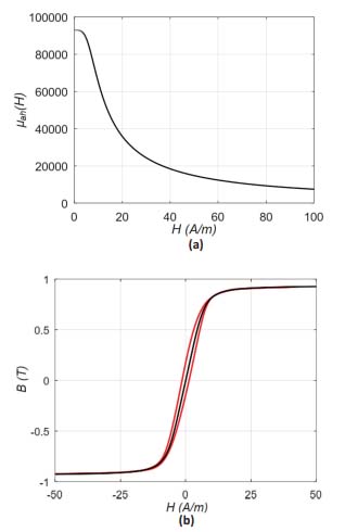
Figure 3.
The results of an anhysteretic curve modeling for the nanocrystalline Fe73.5Cu1Nb3Si15.5B7 alloy: (a) Bah(H) fitting to the quasistatic hysteresis loop B(H) (black – model, red – results of experimental measurements), (b) the results of modeling of its relative permeability dependence μah(H)
Notably, the presented experimental results of the B(H) hysteresis loop measurements don’t reach physical magnetic saturation. However, observed saturation is valid from the technical point of view. For this reason, the presented values of saturation magnetization Ms and saturation flux density Bs should be considered technical saturation values, which are slightly lower than the declared values of physical saturation.
The presented results confirm that the inductive core Vacuumschmeltze W915, made of the Fe73.5Cu1Nb3Si15.5B7 nanocrystalline alloy, exhibits transverse anisotropy introduced during the production process [31]. Moreover, the anhysteretic curve properly reproduces the nonlinear shape of the magnetization curve of the alloy.
The complete gyrator-capacitor circuit used for the modeling is presented in Figure 4. The coil’s driving current waveform, acquired from measurements using the hysteresis graph setup, is provided as a text file Icurr.txt describing the current source I1. The modeled core’s nonlinear anhysteretic magnetization characteristic is tabulated in the description of voltage sources B6 as a function of magnetic permeability μah versus magnetizing field H, according to Equation 6. LTspice enables the even use of long tables, simplifying the precise description of nonlinear anhysteretic magnetization characteristics.
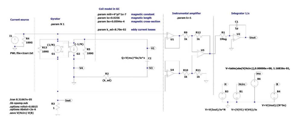
Figure 4.
The complete gyrator-capacitor circuit used for the modeling B(H) hysteresis loop as a function of magnetizing field frequency f for the Fe73.5Cu1Nb3Si15.5B7 (Vitroperm 500F) nanocrystalline alloy
In the gyrator-capacitor model presented in Figure 4, the eddy current losses are modeled by the resistor R2. As previously presented by Chikazumi, the instantaneous power losses per unit volume can be calculated as [32]:
ρ is the material’s resistivity, d0 is the lamination thickness, and β is connected with the core’s geometry. The shape factor β is 6 for laminations, 16 for cylinders, and 20 for spheres [6]. The ked value of resistor R2 can be calculated as [19]:
Vc is the volume of the core, and Ac is the core’s effective cross-section. It should be noted that, since amorphous alloys are typically ribbon-wound cores, the effective cross-sectional area Ac should be estimated based on the core mass and material density. As a result, the value Ac is the value provided by the core’s producer. In addition, considering the physical aspects of the gyrator-capacitor [19], the parameter ked is given in 1/Ω.
The inductor’s output signal is collected by the instrumental amplifier and integrated by the operational amplifier U2, which serves as the integrator. Finally, the values of the magnetic field strength H and flux density B in the nonlinear core of the inductor are calculated using the voltage sources B1 and B4, respectively [20]. The proposed model operates in the transient mode. Time plots of the magnetic field strength H and flux density B in the nonlinear core of the inductor are written to output files, enabling further processing.
Identification of the parameter determining the eddy current loss
For the determination of the optimal value ked of resistor R2, the target function G(ked) was determined as:
Bg–c model(Hi) are the results of modeling the flux density B in the core, using the model presented in Figure 4, for the determined value of resistor R2 equal to ked. The results of the modeling are presented in Figure 5.
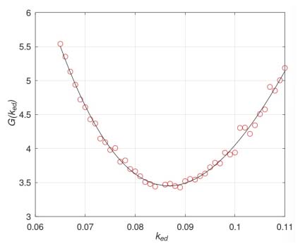
Figure 5.
The results of modeling the target function G dependence on the value of ked for the resistor R2
It can be observed that the value of the function G(ked) exhibits numerical uncertainty. This uncertainty is caused by the measurement uncertainty described in Section 2 and the numerical uncertainty associated with solving ordinary differential equations [5], as stated in the numerical model presented in Figure 4. As a result, it would be difficult to identify the ked value in the optimization process. To overcome this problem, the polynomial response curve method [33] was applied. In this method, the obtained G(ked) dependence results are modeled by a polynomial curve, using the least squares method [34].
The order of the polynomial curve, i equals 3, was determined experimentally, considering the quality Q(i) of regression (least squares value of the differences between the model and results) presented in Figure 6. Finally, the optimal value of parameter ked was estimated as 0.0856 1/Ω.
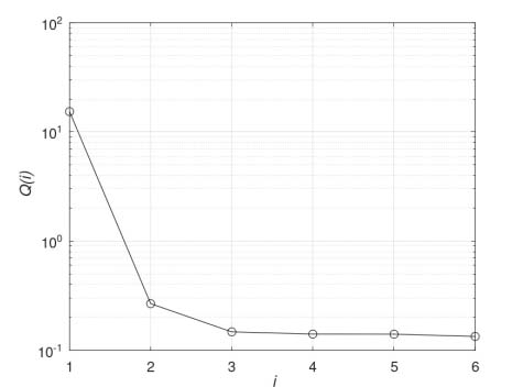
Figure 6.
The dependence of quality Q(i) of regression versus the order of the polynomial used for the approximation
4. Results of modeling
Figure 7 compares the experimental and modeling results using the gyrator-capacitor model. The gyrator-capacitor model represents the frequency dependence of the shape of the magnetic B(H) hysteresis loop of Vacumschmeltze W915 core made of nanocrystalline Vitroperm 500F very well. The goodness of fit is confirmed by the value of the R2 determination coefficient, which exceeds 0.995 for all loops measured at the magnetizing field frequency, ranging from quasistatic to 36 kHz.
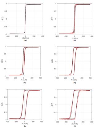
Figure 7.
The comparison of the experimental results and the results of modeling using the gyrator-capacitor model (black – model, red – results of experiments) for the frequency f of the magnetizing field equal: (a) 1 Hz, (b) 2 kHz, (c) 6 kHz, (d) 15 kHz, (e) 26kHz, (f) 36kHz
the parameters of the Vacuumschmeltze W915 core provided by the manufacturer were as follows: The effective cross-section Ac is 5.94⋅10−6 m2; the magnetic path length Lc is 2.56⋅10−3 m, and the material’s generalized resistivity ρ is 1.15⋅10−6 Ωm, because the nanocrystalline ribbon thickness is about 30 μm. As a result, the value of the core’s shape parameter β (given by Equation 10) is 19.5. This value indicates that the layers of the nanocrystalline ribbon in the Vacuumschmeltze W915 core are only partially isolated [35]. This observation aligns with previous experimental measurements of nanocrystalline soft magnetic cores produced by annealing amorphous alloys [36].
Although the described gyrator-capacitor model very accurately represents the frequency dependence of the magnetic B(H) hysteresis loop shape of the Vacuumschmeltze W915 core, the more detailed analysis of the frequency dependence of the coercive field Hc value (presented in Figure 8) clearly shows that the root-square-shaped curve of the modeled Hc(f) curve is not a good fit to previous experimental results. This is connected to the fact that Chikazumi’s model (given by Equation 9) is simplified [32] and doesn’t describe all effects related to eddy current power losses in the laminated materials [37]. A more detailed functional model of the Hc(f) curve and its implementation in the gyrator-capacitor model should be considered as a goal of further research.
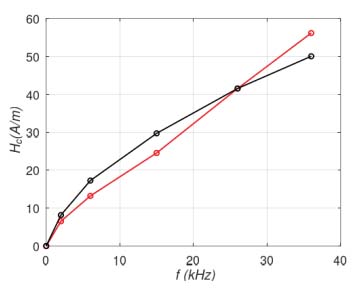
Figure 8.
The frequency f dependence of the coercive field Hc value (black – model, red – results of experimental measurements)
5. Conclusions
The presented results confirm that the modeling results based on the gyrator-capacitor model with eddy current losses, as described by a resistor, are in agreement with other experimental measurements. In the case of the Vacuumschmeltze W915 core made of nanocrystalline Fe73.5Cu1Nb3Si15.5B7 alloy (Vitroperm 500F), this agreement is confirmed by the value of the R2 determination coefficient, which exceeds 0.995 for all loops measured for the magnetizing field frequency, from quasistatic up to 36 kHz. In addition, considering the core’s parameters provided by the manufacturer, the value of the core’s shape parameter β was estimated as 19.5, indicating that the layers of the nanocrystalline ribbon in the Vacuumschmeltze W915 core are only partially isolated.
On the other hand, the frequency dependence of the coercive field Hc value indicates that the root-square-shaped curve Hc(f) exhibits limited fit to experimental results. As a result, further research of more detailed functional models of the Hc(f) curve and their implementation in the gyrator-capacitor model should be conducted.