

1. Introduction
The worldwide energy demand is constantly being enhanced owing to population growth and industrialization [1,2]. Traditional fossil fuels like coal, oil, and natural gas are the main sources of energy, although their usage has led to various issues such as environmental pollution and contribution to climate change through greenhouse gas emissions [3, 4]. To address these issues, there has been a rising emphasis on developing and utilizing renewable energy sources (RESs) such as solar, wind, and geothermal power [5, 6]. Among these various RESs, photovoltaic (PV) technology has emerged as a promising topology due to its various advantages, which generate electricity without producing greenhouse gas emissions or other forms of ecological pollution, thus generating a clean and sustainable energy solution [7–9]. Though the output voltage of PV is lower because of its intermittent nature, direct current (DC), DC converters are essential for efficiently converting variable DC output of the PV modules to the increased level of energy required for grid applications [10]. In this context, various traditional converters used in current studies such as Boost [11], Buck-Boost [12], and Cuk [13] converters provide step-up and step down voltage with better voltage gain. Nevertheless, each converter topology has its own advantages and drawbacks such as poor efficiency, high cost, complexity, and switching stress [14,15]. Henceforth, the proposed topology employs a single-ended primary inductor converter (SEPIC) to overcome these challenges by attaining high efficiency with minimized switching stress and ripple current.
In contrast, maximum power point tracking (MPPT) techniques are specifically designed to optimize power output from solar panels by continuously adjusting to varying conditions, making them more effective in maximizing energy extraction. Compared to proportional integral (PI) and fractional order sliding mode control controllers, intelligent MPPT provides superior adaptability and efficiency under fluctuating input conditions, highlighting its advantage in energy harvesting applications [16–20]. To improve the performance of tracking efficiency, various traditional topologies have been developed, which are illustrated in Table 1 below.
Table 1.
Survey related to the traditional MPPT approaches
| References | Methodology | Advantages | Limitations |
|---|---|---|---|
| Shaik rafi kiran et al (2022) [21] | artificial neural network (ANN) based MPPT | It achieves better tracking efficiency with minimized oscillation of MPP. | However, this system applicable for partially shaded PV system. |
| Faizan Mehmood et al (2020) [22] | Fuzzy-based MPPT | At the period of transient condition, this technique attains better performance with efficient power delivery. | Nevertheless, it has steady state oscillations and system complexity. |
| Sara et al (2021) [23] | ANFIL-based MPPT | It has higher accuracy, faster response with better tracking. | However, due to increasing number of rules, the system complexity is enhanced. |
| Chaoping rao et al (2022) [24] | Perturb observe (P&O)-Based MPPT | It attains minimized steady-state error with better tracking efficiency. | Nonetheless, the fluctuation around MPP and complexity leads to degradation of system performance. |
| Pawan Kumar Pathak et al (2021) [25] | modified incremental conductance (INC)-based MPPT | MINC attains high tracking efficacy with effectual convergence speed. | However, execution time needs to be considered in further studies. |
To overcome the limitations obtained in the traditional MPPT topologies, the proposed work incorporates a novel cascaded artificial neuro fuzzy inference system (ANFIS)-radial basis function neural network (RBFNN)-based MPPT, which has the advantages of enhancing MPPT accuracy and robustness under varying environmental conditions with rapid convergence speed and execution time. The foremost contributions of the proposed work are illustrated below,
Implementing a PV-based SEPIC to efficiently handle an extensive input voltage range, ensuring optimal power conversion system, even under varying solar conditions.
The cascaded ANFIS–RBFNN-based MPPT approach is introduced for extracting the highest power from the PV system, resulting in improved MPPT accuracy with minimal computational time.
Employing PI controller for ensuring precise regulation of the single phase inverter output to synchronize with the grid frequency and voltage.
Section 2 describes the proposed system modeling; Section 3, the outcomes from the MATLAB/Simulink for the developed work is discussed with a comparative analysis. Further, in Section 4, conclusions about the proposed system are discussed by showing the importance of the proposed system.
2. Proposed Modeling
PV systems have gained significant importance in the RES, as it offers a clean and sustainable source of electricity. However, the sporadic nature of solar radiation and the nonlinear characteristics of PV systems pose challenges in maintaining a stable and efficient power supply to the grid. To address these challenges, this research explored SEPIC with the novel cascaded ANFIS–RBFNN-based MPPT topology, which provides an enhanced output voltage with better tracking performance. The proposed work block diagram is shown in Figure 1 below.
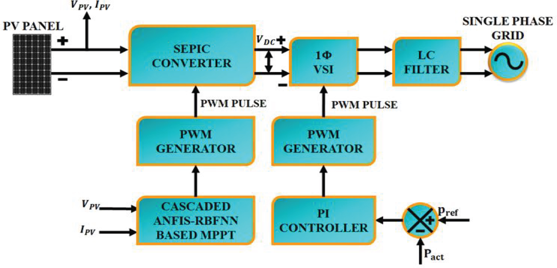
Figure 1.
Block diagram of the proposed work
In this work, SEPIC has been developed for maximizing the low-output voltage of a PV system for the essential level for a grid system. On the other hand, the MPPT approach is used for tracking optimal energy from the PV modules; thus the cascaded ANFIS–RBFNN-based MPPT topology has been developed, which leverages the strength of each approach to enhance control precision, robustness, and maximum energy harvesting from the solar module. The tracked output is fed to the Pulse Width Modulation (PWM) generator for producing required pulses for the switching operation of the SEPIC. A stable DC-link voltage is delivered to the single-phase Voltage Source Inverter (VSI) for converting the DC-AC supply; it is regulated by the PI controller for attaining grid synchronization. Finally, the required level of energy is given to the grid system without any disturbances.
2.1. Modeling of the PV System
The PV system generates electricity directly from sunlight, a free and abundant RES. Unlike fossil fuels, this energy production does not release greenhouse gases or other pollutants, making a clean and ecological friendly energy source. An equivalent circuit of PV module is represented in Figure 2.
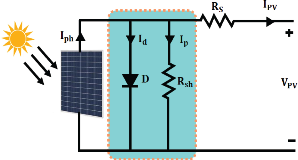
Figure 2.
Circuit diagram of a PV module
Kirchhoff’s current law is applied as follows [21]:
The Id and Ish are derived as follows:
where I0 denotes reverse saturation current, Rsh, Rp, and Rs specifies shunt, series, and parallel resistances, and VT indicates thermal voltage. The following equations express I0 and VT:Here, ∝ indicates diode ideality constant, n specifies the diode’s ideality factor, Ns and shows the panel linked in series, Vop,cct represents open-circuit voltage, T shows the temperature= 1.38 × 10⁻³, and q denotes the charge of electron = 1.6 × 10⁻¹⁹, respectively. Moreover, the low output power is obtained from PV owing to its ecological changes; thus, SEPIC is employed in this study for boosting the voltage as follows.
2.2. Modeling of SEPIC
SEPIC is a popular choice for interfacing the PV system-fed grid system due to its ability to operate in both step-up and step-down modes, allowing for efficient power transfer. The circuit of SEPIC is represented in Figure 3, which shows two inductors, a switch, two capacitors, and a diode, respectively. Furthermore, the proposed converter operates in two modes, as specified in Figure 4.
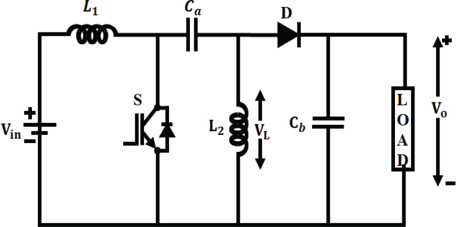
Figure 3.
SEPIC converter circuit diagram
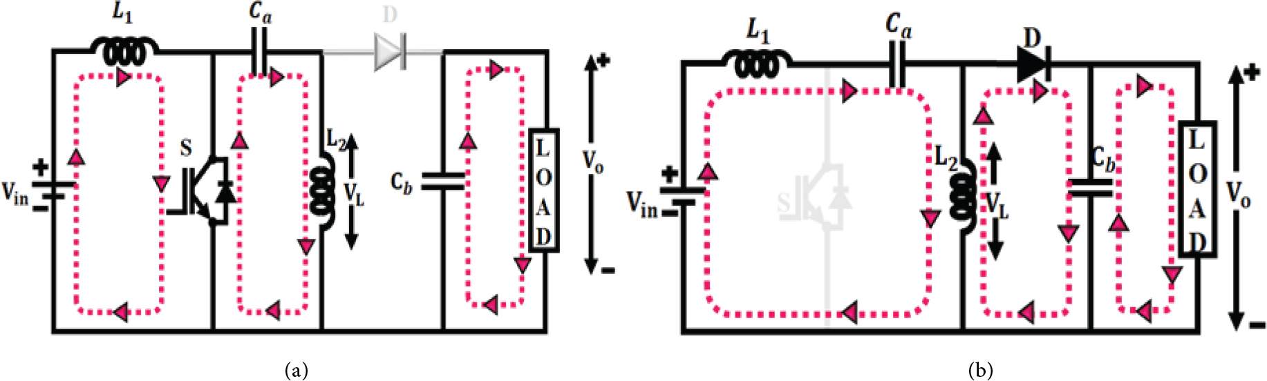
Figure 4.
Modes of operation
The following expression shows the average voltage:
The sum of the average currents is given as follows:
The duty cycle of SEPIC is defined as:
The minimum duty cycle is expressed as:
Mode 1 (ON state): When switch S1 is in the ON condition, the current in L1 becomes negative during the current increases; the diode does not conduct in this state. The capacitor discharge during both L1 and L2 gets charged, as represented in Figure 4(a).
Mode 2 (OFF state): When the switch is in the OFF state, the diode function is forward-biased, an output gets energy from L1 during induction, and L1 charges the capacitor Ca, as illustrated in Figure 4(b), respectively. Also, the switching waveform for the proposed SEPIC is illustrated in Figure 5.
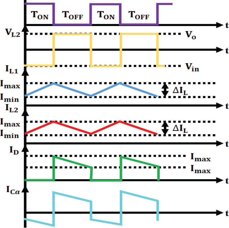
Figure 5.
Switching waveform for the proposed converter
The ripple current flowing through inductors La, Lb is equal to
The inductor value is calculated as
The output capacitor is given as
Here, the switching frequency (fsw) is taken as = 10KHz.
Therefore, the duty cycle range of inductors L1, and L2 and capacitors Ca, Cb are defined using the foresaid equations. The following section explains the cascaded ANFIS–RBFNN-based MPPT for extracting optimal power from the PV system.
2.3. Modeling of Cascaded ANFIS–RBFNN Based MPPT ANFIS-based MPPT
The ANFIS-based MPPT is a powerful technique that combines the strength of fuzzy logic control and ANN, which maximizes the power of PV systems, as specified in Figure 6. This approach is particularly well-suited for dealing with the highly nonlinear and complex relationship between the parameters of PV. In ANFIS, the fuzzy inference system (FIS) is responsible for modeling the nonlinear relationship between the PV system’s output and desired output using a set of if-then rules and membership functions. On the other hand, the ANN is employed to automatically tune the parameters of the FIS, such as membership function and rules based on the available training data. Through the back propagation algorithm, ANN learns the optimal FIS parameters, reducing error between actual and desired output. The multilayer feed-forward networks are described by the following mathematical equation:
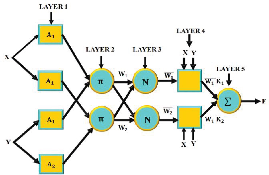
Figure 6.
Structure of ANFIS
The following equations express K1, K2, and K,
where pj, rj, and bj denote the membership function, respectively.RBFNN-based MPPT
The nonlinear mapping is performed using an RBFNN, unlike the error backpropagation learning model of conventional neural networks, RBF networks employ a learning process that is equivalent to solving a linear problem. The hourly requirement oscillation serves as input for the RBFNN network training, which has three types: input, hidden, and output layers, as specified in Figure 7. The input layer is the top layer, which is carried out by the input data source nodes. The second layer produces radial-based processes. The third layer is the output layer, which specifies the nonlinear combination of neural parameters and input radial basis function. Overall this RBFNN’s primary goal is to forecast the PV system’s maximum power.
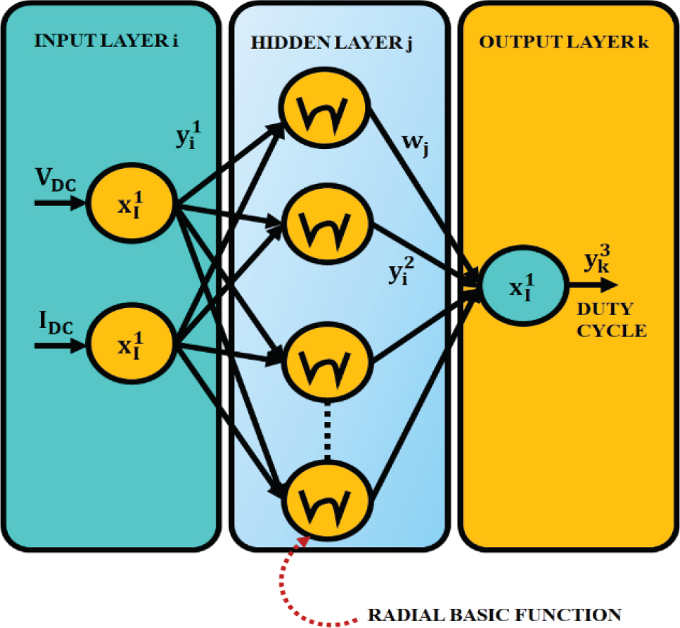
Figure 7.
RBFNN architecture
Step: 1 Create initial input vectors based on variables such as voltage, current, and power, which are adjusted based on the network’s output power requirements.
Step: 2 After the initialization process, the system generates its initialized input parameters at random [22].
Here, Ppd specifies the power demand.
Step: 3 By reducing the error function, which is provided below, fitness is assessed.
where the desired and target output demand is denoted as d0D and t0D.Step: 4 The Gaussian activation function of RBFNN yields the RBFNN output, which is provided as follows:
where ξ specifies the Gaussian activation function, and yp denotes the p-th input sample, respectively.The number of nodes in the hidden layer specifies h. Moreover, by combining this two approaches, the performance of tracking efficiency is enhanced, as described below.
Cascaded ANFIS–RBFNN-based MPPT
The cascaded ANFIS–RBFNN-based MPPT combines two powerful techniques to improve the efficiency of capturing maximum power from solar panels. First, ANFIS uses fuzzy logic and neural networks to adaptively adjust its rules based on changing conditions, helping to predict and optimize power output. Second, the RBFNN provides precise function approximation by using radial basis functions to finetune the tracking process. Together, this cascaded approach enhances the MPPT algorithm’s ability to rapidly and accurately find the optimal power point, resulting in better performance and energy extraction compared to traditional methods. The developed cascaded ANFIS–RBFNN-based MPPT system flowchart is indicated in Figure 8, which shows that the system measures the solar irradiance, which is a crucial input parameter for the MPPT algorithm. It also measures the voltage and current from the PV system, which are used as inputs to the developed MPPT algorithm. The next step is to detect any abrupt changes in the solar irradiance, as these changes affect the optimal operating point of the PV system. If an abrupt change is detected, the system sets a new operator voltage to ensure the PV system is operating at its highest point. The core of the MPPT algorithm is the ANFIS-RBFNN-based MPPT block. This combines the ANFIS and RBFNN to track the MPP of PV system efficiently, even in the presence of abrupt changes in solar irradiance. The ANFIS component provides the fuzzy-logic-based decision making, while the RBFNN component handles the nonlinear mapping between the input parameters and the optimal operating voltage. By combining this, the overall efficiency, reliability is significantly improved, creating more viable and improved performance of SEPIC.
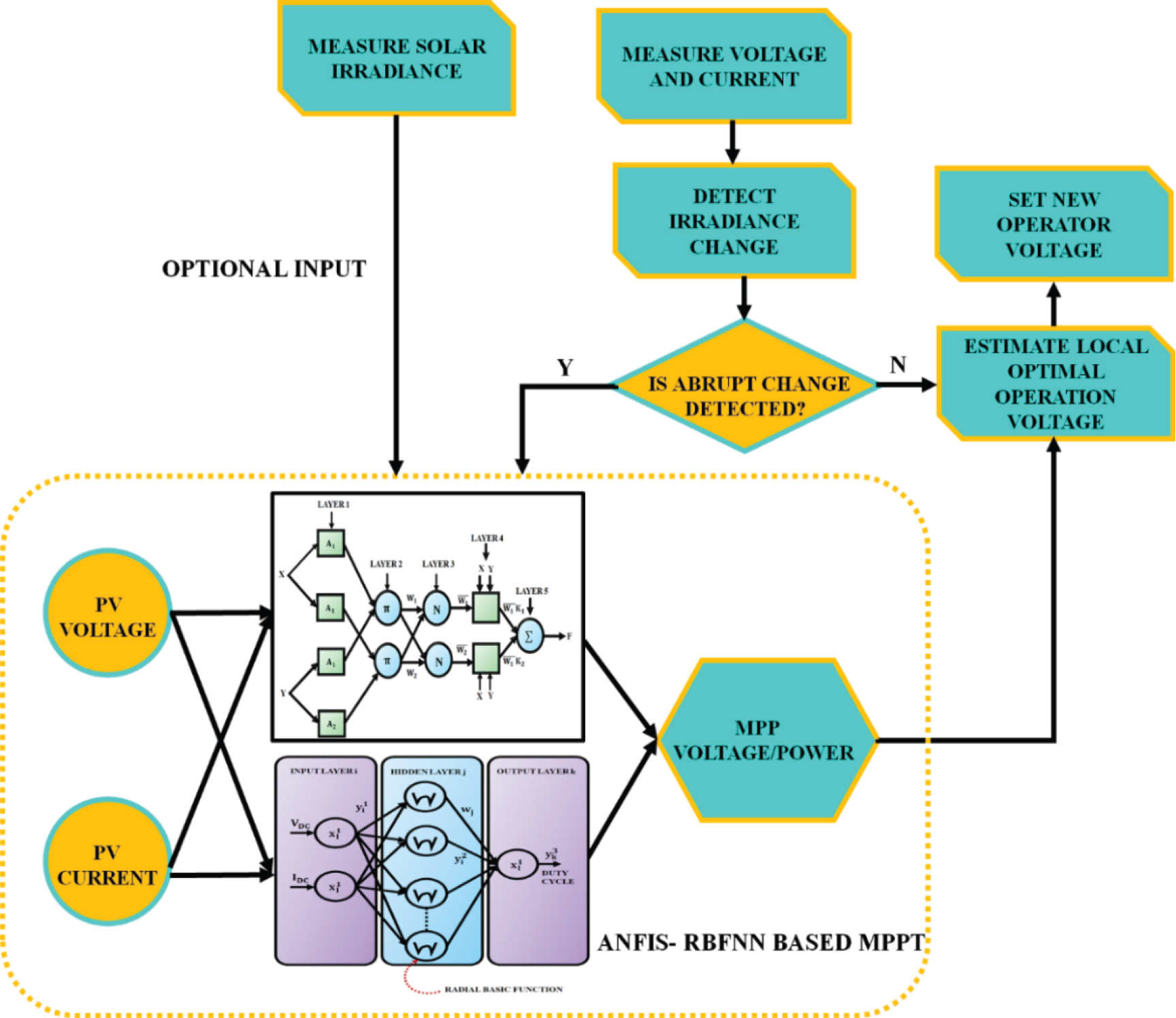
Figure 8.
Proposed cascaded ANFIS–RBFNN-based MPPT
By utilizing the proposed approach, the optimal energy from the PV system is efficiently tracked with greater tracking efficiency, execution time, and convergence speed. Moreover, the tracked and enhanced power is given to the single-phase VSI for converting the DC-AC supply to distribute power to the single-phase grid system. Also, the inverter is efficiently controlled with the aid of the PI controller for grid synchronization.
3. Results and Discussion
In this work, a SEPIC-based cascaded ANFIS–RBFNN approach is developed for grid applications. The proposed system is validated in MATLAB/Simulink for validating the effectiveness of the developed system. Additionally, the comparative assessment is carried out with other traditional topologies for showing the importance of the developed work. In Table 1, parameter specifications for the proposed system are illustrated.
Table 2.
Parameter Specifications of Proposed System
| Parameter | Description |
|---|---|
| PV system | |
| Open circuit voltage | 37.25V |
| Short-circuit current | 8.95A |
| Series-connected solar panel | 2 |
| Parallel-connected solar PV cell | 25 |
| Maximum power voltage | 29.95V |
| Maximum current | 8.35A |
| SEPIC | |
| Switching frequency | 10kHz |
| Ca, Cb | 4.7μF |
| L1, L2 | 1 mH |
(a) Case 1. Varying Temperature and Varying Irradiation
The solar module waveform is illustrated in Figure 9. The temperature of the solar panel varies slightly during the initial time, and after 0.2 s it is stabilized at 45°C, as specified in Figure 9(a). Consequently, the irradiation of the solar panel is maintained constantly at 1000(W/Sq.m) after the fluctuation up to 0.2s, as specified in Figure 9(b). Also, the voltage of the solar panel for the proposed work attains the stabilized voltage at 48V after 0.2s, as illustrated in Figure 9(c).
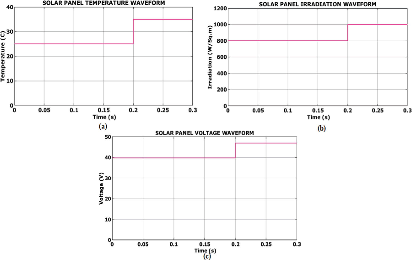
Figure 9.
Solar module waveform for case 1. (a) Temperature; (b) irradiation; (c) voltage
The proposed SEPIC waveform is illustrated in Figure 10. The input current waveform indicates that the input current oscillates highly during the starting period, and after 0.22s, the constant current is maintained at 0.8A, as specified in Figure 10(a). From Figure 10(b), it is observed that the converter output voltage is stabilized at 300V after 0.25s. Similarly, the converter output current has high oscillation during the initial time, and after 0.05s a constant output current is obtained at 25A with fluctuations.
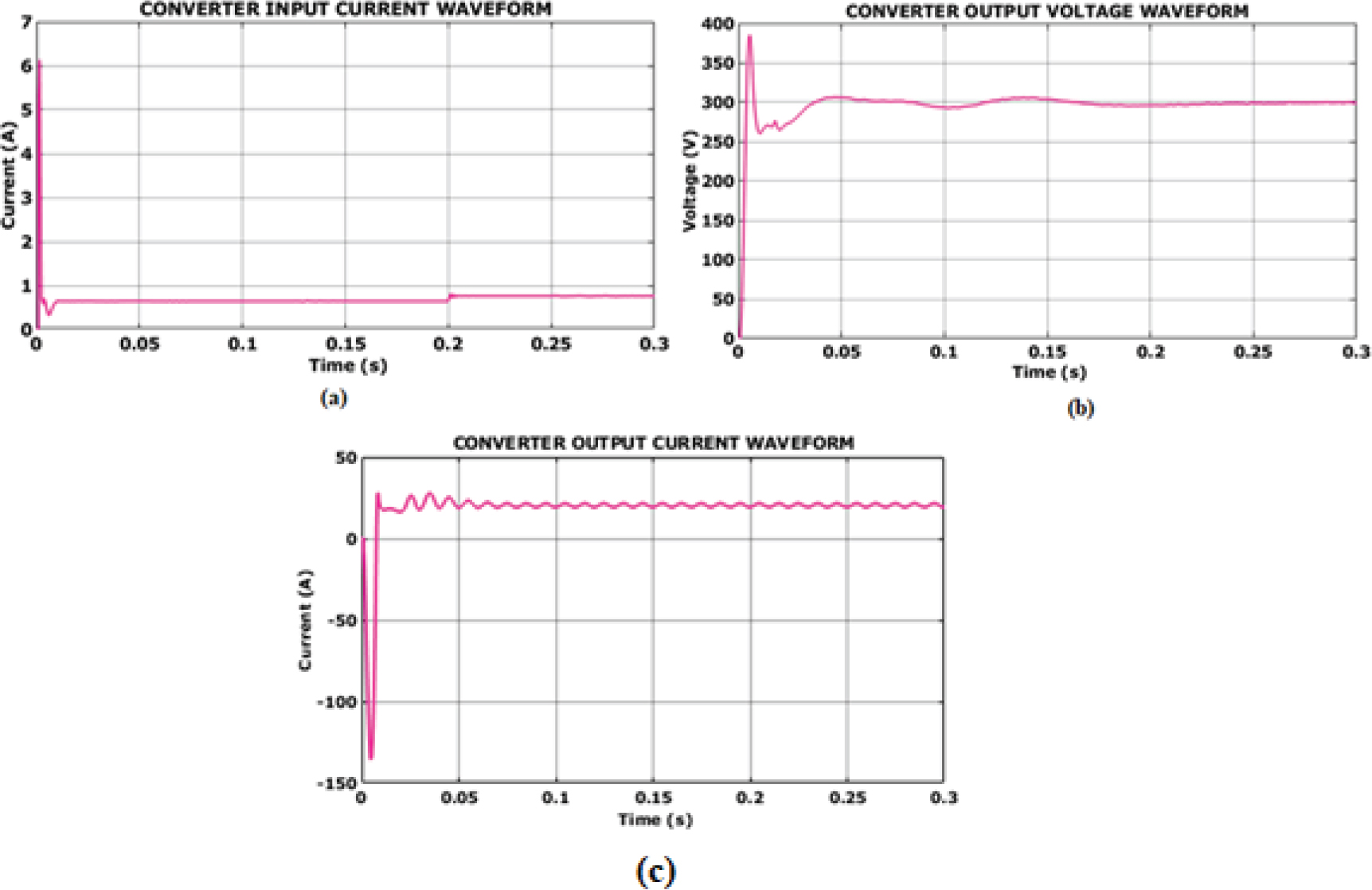
Figure 10.
Converter output waveform for case 1
The grid waveform is indicated in Figure 11. The grid voltage waveform illustrates that the grid voltage is stabilized at 230V without any distortions, as illustrated in Figure 11(a). Likewise, the current waveform specified in Figure 11(b) indicates that the grid oscillates slightly, and after 0.05s it stabilizes at 4A. Moreover, the in-phase waveform is specified in Figure 11(c), where it can be observed that the voltage and current stabilize at 230V and 4A, respectively.
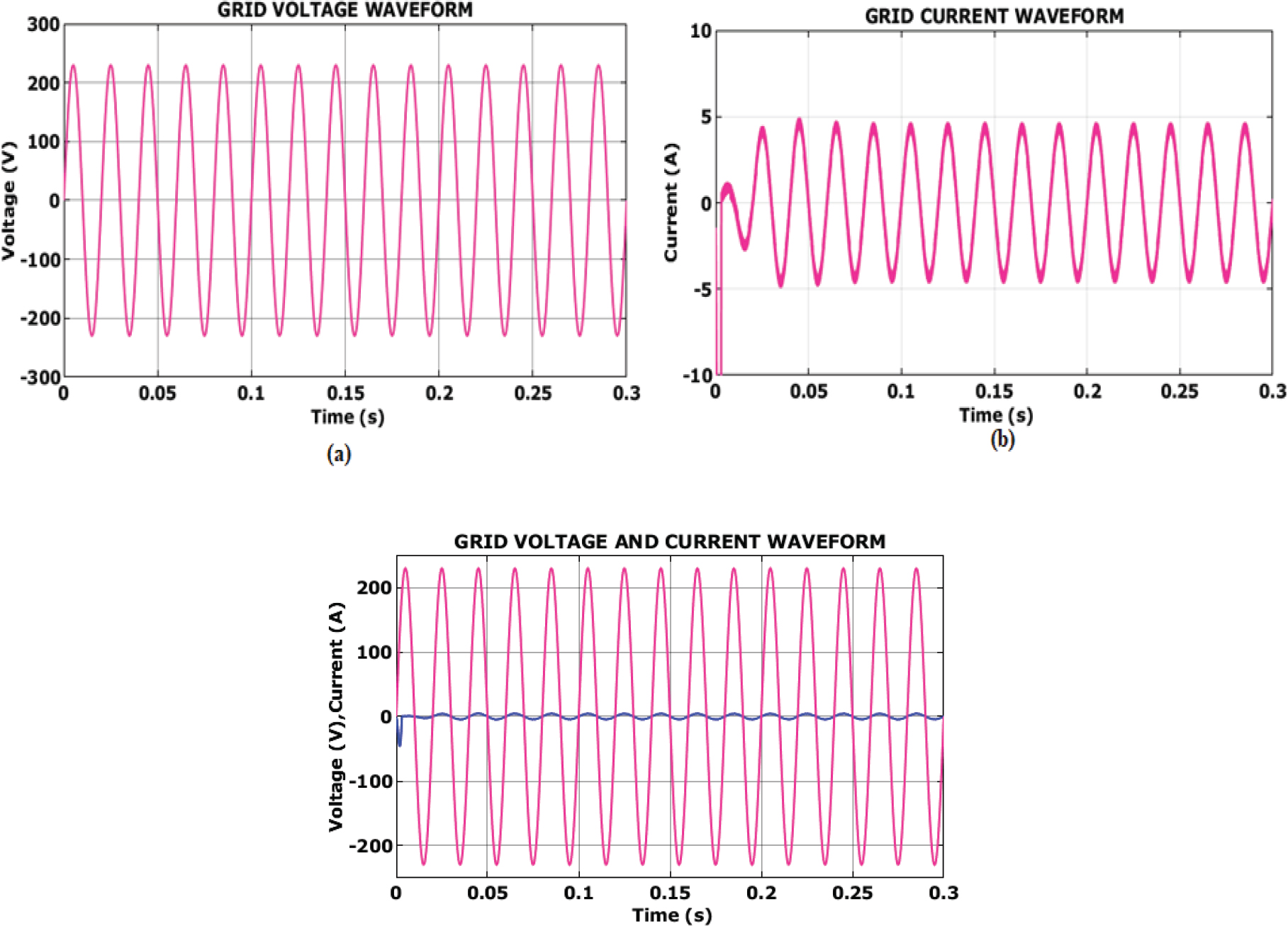
Figure 11.
Grid waveform. (a) Voltage; (b) current; (c) in-phase voltage and current waveform
The real and reactive power for the developed work is illustrated in Figure 12. The stabilized real and reactive power results in the superior performance of the proposed system.
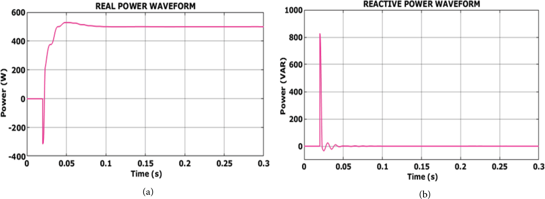
Figure 12.
Real and reactive power waveform
(b) Case 2. Constant temperature and constant irradiation
Figure 13 represents the solar panel waveform for case 2, which shows that the temperature of the solar panel gets constantly stabilized at 35°C, as indicated in Figure 13(a). Similarly, the irradiation waveform illustrated in Figure 13(b) shows that the irradiation is maintained at 1000(W/Sq.m). The voltage of solar panel attains stability at 48V in the case 2 condition, as indicated in Figure 13(c).
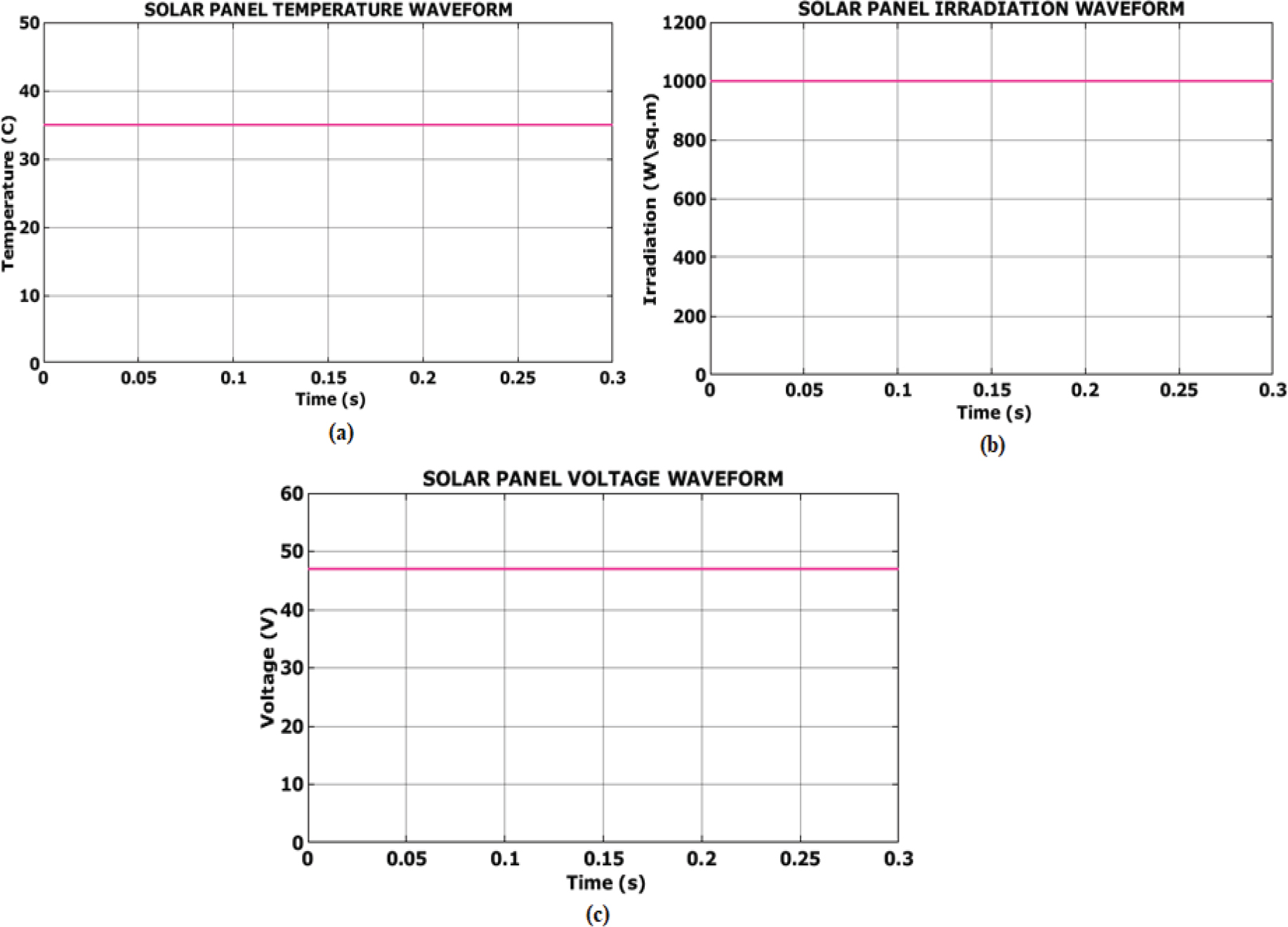
Figure 13.
Solar panel waveform for case 2
The converter waveform for the case 2 condition is represented in Figure 14. As specified in Figure 14(a), the converter input current oscillates highly during the initial period, and after 0.02s, the constant current is attained at 0.8A. Moreover, the output voltage waveform, indicated in Figure 14(b), shows that the voltage is constantly maintained at 300V after facing high fluctuation up to 0.25s. The converter output waveform illustrated in Figure 14(c) indicates that the output current fluctuates highly, and after 0.05, s, it gets stabilized with distortions.
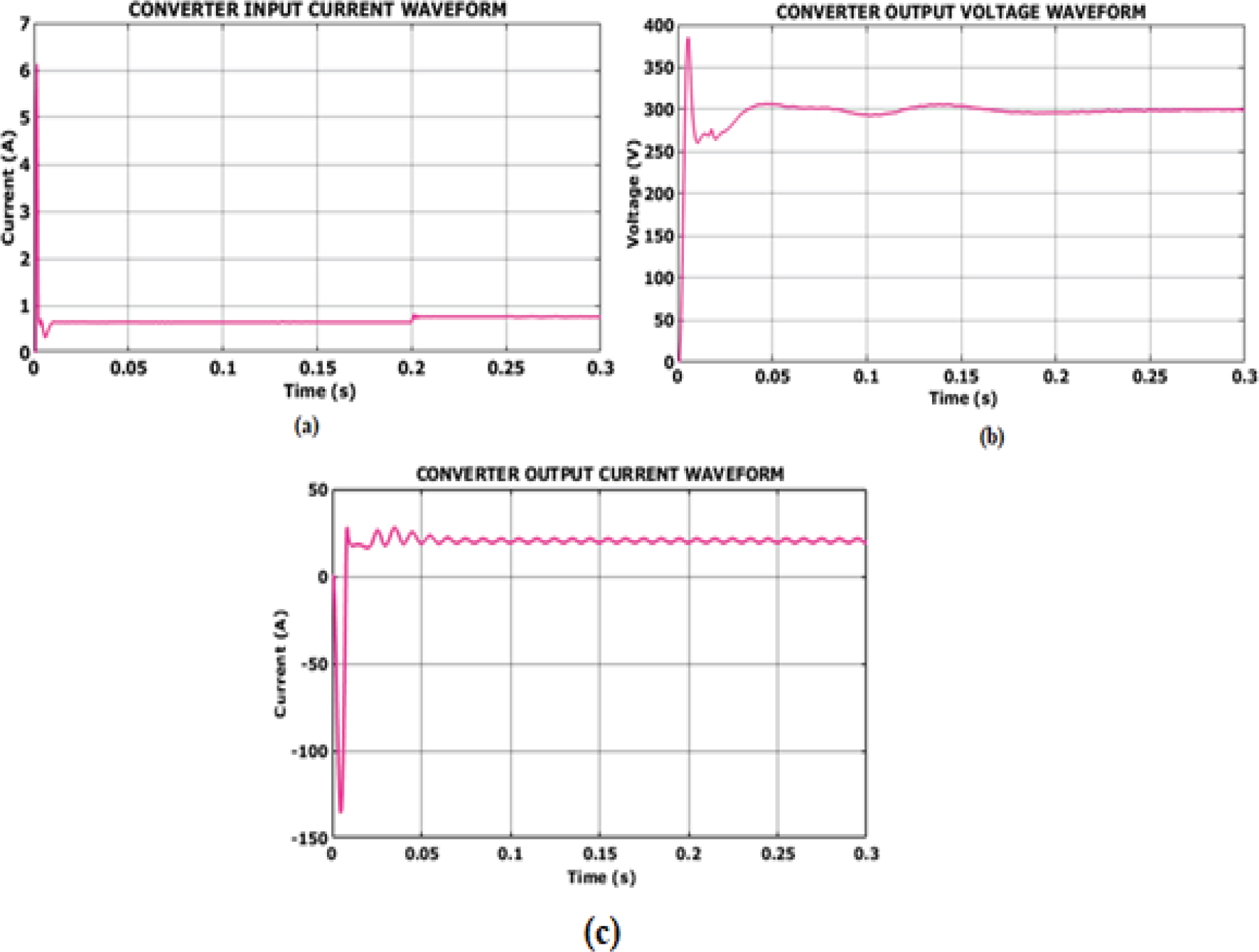
Figure 14.
Converter waveform for case 2
(c) Case 3. Varying Temperature and Constant Irradiation
The case 2 condition for solar module waveform is represented in Figure 15. Figure 15(a) illustrates the varying temperature condition, where the temperature oscillates up to 0.2s and afterward is maintained gradually at 35°C. Likewise, the irradiation waveform illustrated in Figure 15(b) shows that the irradiation is maintained at 1000(W/Sq.m). Also, Figure 15(c) indicates that the solar panel voltage oscillates up to 0.2 s; after that, it stabilizes at 48V.
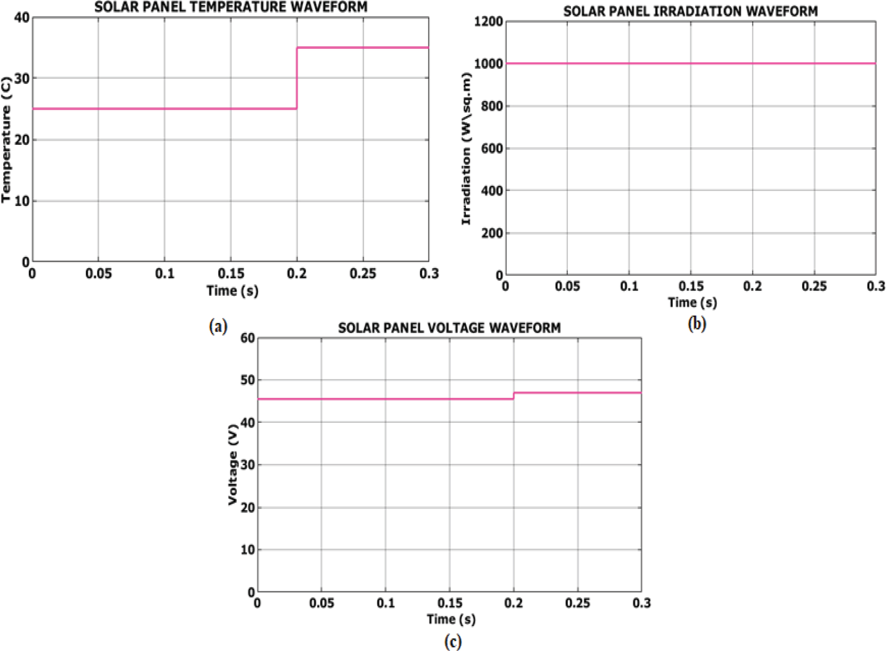
Figure 15.
Solar panel waveform for case 3
As shown in Figure 16(a), during the first 0.02 s, the converter input current oscillates greatly before reaching 0.8A of steady current. Furthermore, Figure 16(b) shows that the output voltage waveform is progressively maintained at 300V following a significant fluctuation that lasted for 0.25 s. The converter output current waveform shown in Figure 16(c); it fluctuates greatly during the initial time, and after 0.03 s, it is maintained at 25A with slight distortions.
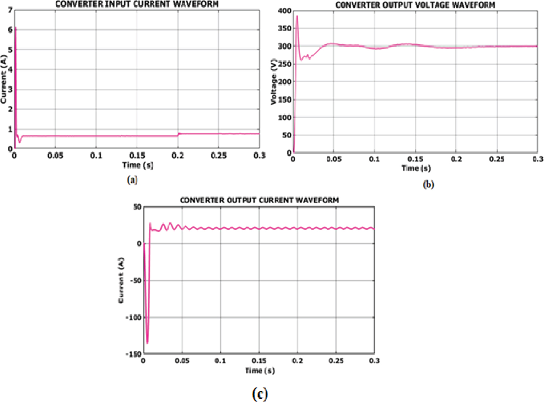
Figure 16.
Converter waveform for case 3
(d) Case 4. Constant Temperature and Varying Irradiation
The solar panel waveform for scenario 4 is shown in Figure 17, where it can be noted that the solar panel’s temperature steadily stabilizes at 35C, as represented in Figure 17(a). Figure 17(b) illustrates that the solar panel’s irradiation is stabilized at 1000(W/Sq.m) following a variation of up to 0.2s. Additionally, as illustrated in Figure 17(c), the solar panel voltage reaches astabilized value at 48V after 0.2s.
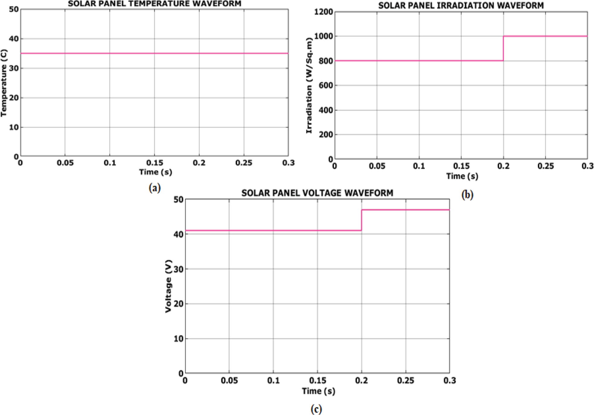
Figure 17.
Solar panel waveform for case 4
The converter waveform for the final condition is shown in Figure 18. As seen in Figure 18(a), the converter input current oscillates greatly in the first period before reaching 0.8A of steady current after 0.02 s. Additionally, the output voltage waveform illustrated in Figure 18(b) demonstrates that the output voltage is constantly maintained at 300V following a strong fluctuation lasting up to 0.25s. The output current fluctuates greatly, as seen by the converter output waveform represented in Figure 18(c), and then stabilizes after 0.05s at 25A with distortions.
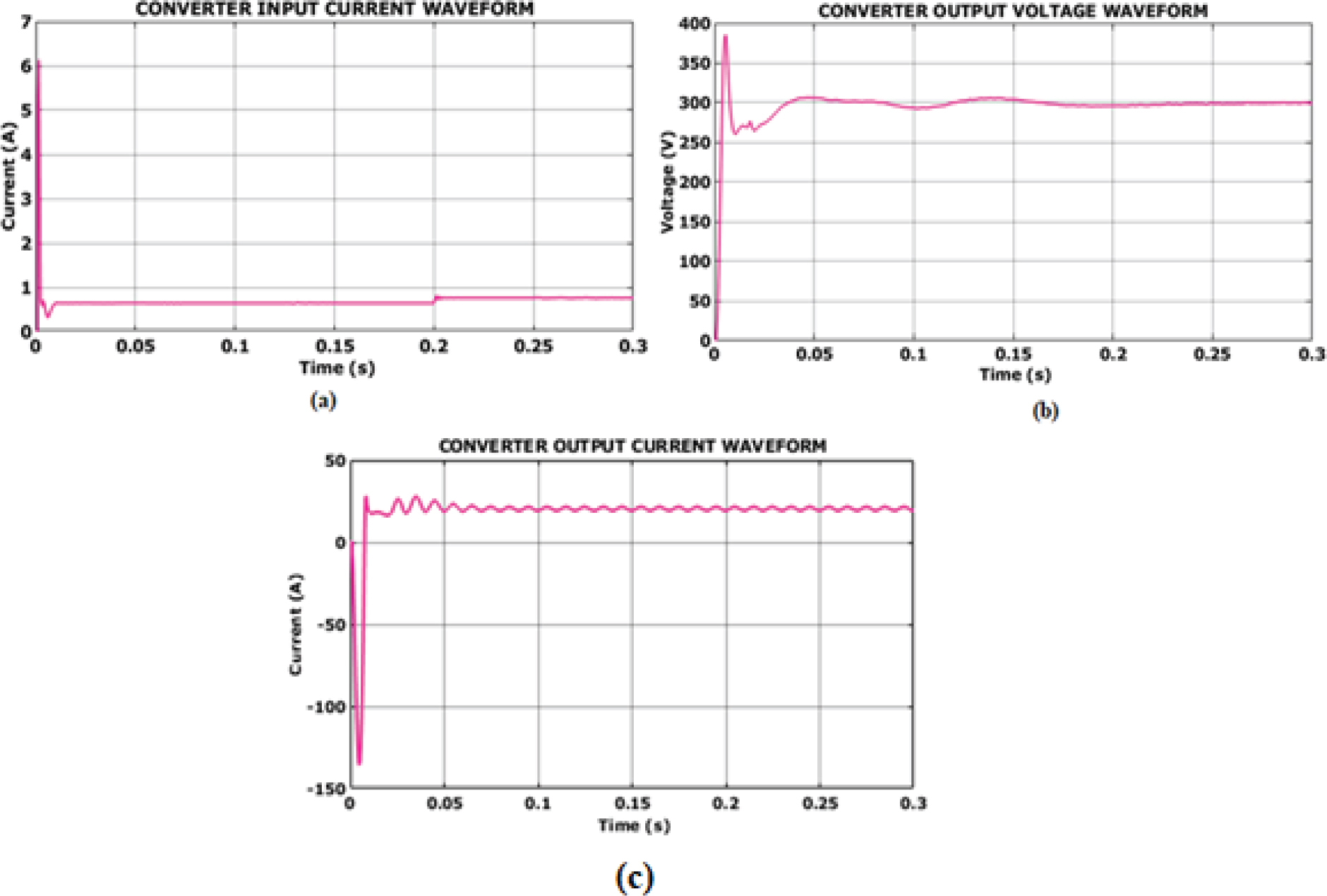
Figure 18.
Converter waveform for case 4
The THD waveform for the developed work is specified in Figure 19, where it is observed that the THD value of 1.16% is obtained. Thereby the performance of the developed system is efficiently enhanced.
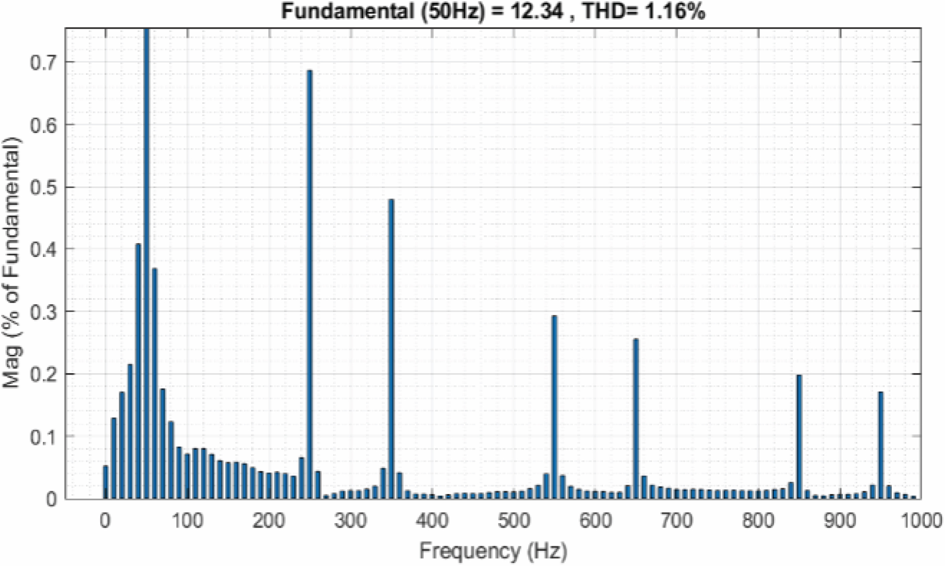
Figure 19.
THD waveform for the proposed work
The tracking efficiency for various MPPT approaches is compared with the introduced cascaded ANFIS–RBFNN-based MPPT, as demonstrated in Figure 20. From the graph, it is evident that the developed MPPT approach accomplishes high tracking efficiency of 99.61% compared to the other topologies, as referred to in [28–30].
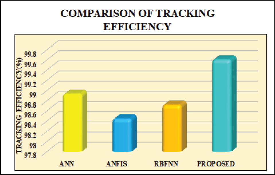
Figure 20.
Comparison of tracking efficiency
Table 3 represents the comparison of THD for various traditional converters. The developed SEPIC reaches the lowest THD value of 1.89% compared to the other approaches.
Table 3.
Comparison of THD for Various Converters
| SI. No | Converters | THD (%) |
|---|---|---|
| 1. | Boost [11] | 6.42 |
| 2. | Buck-Boost [12] | 3.43 |
| 3. | Cuk [13] | 4.41 |
| 4. | Proposed SEPIC | 1.16 |
The proposed cascaded ANFIS–RBFNN-based MPPT technique is compared with conventional MPPT approaches for convergence speed and execution time in Figure 21. From the graph, it is obvious that the cascaded approach attains high convergence speed and minimized execution time compared to traditional MPPT topologies.
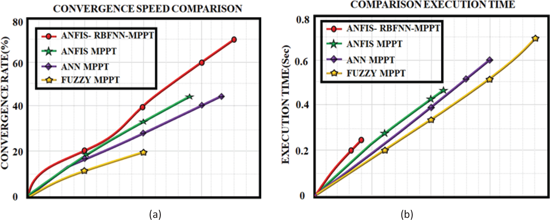
Figure 21.
Comparison of (a) convergence speed and (b) execution time
4. Conclusion
The proposed research work introduced SEPIC-based novel cascaded RBFNN-based MPPT for grid applications. The proposed SEPIC effectively interfaces the PV array with the grid, providing stable voltage regulation. The integration of cascaded ANFIS-RBFNN-based MPPT enables efficient tracking of the MPPT under varying ecological conditions, maximizing the energy harvested from the PV system with high tracking efficiency. The developed system is validated through MATLAB/Simulink, and the outcomes are compared with other traditional approaches, showing the superiority of the developed system. From the comparison results, the effectiveness of a novel cascaded ANFIS–RBFNN based MPPT exhibits superior tracking efficiency of 99.61% capabilities, convergence speed, execution time with improved steady-state and dynamic responses. Also the SEPIC achieves a low THD value of 1.16% compared to the others. Thereby, the enhanced and tracked power is efficiently delivered to the grid system without any disturbances.