

Driven by the development of deep neural networks, notable advances in Artificial Intelligence (AI) have been evident in recent years, revolutionizing fields such as image processing, voice recognition and natural language processing; making these systems increasingly present in different domains and as such in daily life [1, 2].
Despite being increasingly present, these models act as “black boxes”, which makes them incomprehensible to humans, making it impossible to understand their internal reasoning and the causes that led the system to its prediction. Given the need to interpret and understand AI models, the field of explainable artificial intelligence (XAI) is developed [3].
XAI seeks to create techniques to make AI models more interpretable and understandable to humans, generating explanations for how they reach their conclusions and predictions. For example, you can show the most influential input features or design more transparent hybrid models. Although there is a tradeoff between performance and transparency, a better understanding of how the system works can correct its shortcomings. XAI is one of the key requirements for implementing responsible AI, a methodology for large-scale implementation of AI methods in real organizations with fairness, model explainability, and accountability [3].
In recent years, several techniques have emerged to explain the predictions of these systems, highlighting LIME [4], SHAP [5], Integrated Gradients [6] and Time Series Saliency (TSSaliency) [6].
This paper presents a neural network for predicting electricity generation from a photovoltaic park and also makes a comparison between different methods for explaining regression networks, with the aim of offering a guide on the options available when it comes to implementing explainable solutions in artificial intelligence projects for the prediction of neural networks [1].
Explainability is the basis for humans to trust and understand the decisions made by machine learning models, as it offers clarity and understanding about the internal workings of these models, facilitating their responsible use and increasing their effectiveness in various scenarios.
There are two important aspects regarding explainability. The first aspect, understanding the cause of the decision, allows us to understand the specific factors that led the model to make a specific prediction. This usually involves being able to identify the most relevant characteristics and their impact on the decision. The second aspect, the ability to predict future results, implies that by understanding the causes of previous decisions, it is possible to reason and predict the future results of the model more accurately [1, 7].
In the last half decade the XAI has begun to gain some strength as a research field and consequently more tools are being developed for this purpose, some of the most important are: AIX360 [8], inter-pretML [9], SHAP [10], AlibiExlain [11], Captum [12], iNNvestigate [13], explAIner [14], LIME [4], OmniXAI, among many more. Each one has its own approach to different types of data and network architectures.
There are two main approaches to explainability: models interpretable by nature and explanation methods. Models interpretable by nature are based on the design of models that, due to their own structure, are easy for humans to understand. Some examples are: decision tree models, simple linear regression, k-nearest neighbors (k-NN), and Naive Bayes. They have a simple functional form and little complexity that allows the prediction logic to be understood intuitively.
Explanation methods are techniques developed specifically to generate explanations about the functioning of black box models such as neural networks, Support Vector Machines, Random Forest, et al. Examples include: variable importance analysis, rough rule estimation, heat maps, and selecting representative examples. Each method takes a different approach to opening the black box and explaining the model’s decision making.
Both interpretable models by design and subsequent explanation methods are useful and complement each other to improve the transparency, trust and adoption of artificial intelligence systems. A hybrid approach using both approaches is ideal for many real-world applications [15].
Explanation methods are divided into two categories: local methods and global methods. These differ in what they explain (individual predictions or the model as a whole.)
Global methods are generally used to describe how a model works with the inspection of the model’s concepts. This refers to the ability to ask, “What common features were generally associated with the images assigned to this particular class?” But it is difficult to directly find a global explanation for a black box model.
Local methods explain individual decisions made by a model, providing information about why the model selected a specific option for a particular case. These methods are based on the context of the input example and help understand the relationship between the specific characteristics of that example and the prediction [16].
The choice between these methods depends on the nature of the question you seek to answer. However, both global and local are essential to ensure fairness and prevent bias in AI models, thus offering a broader and more detailed understanding of how these models make their decisions.
Post-hoc explainability takes a trained model as input and extracts the underlying relationships that the model learned by building a white box surrogate model. By doing so they only generate an approximation of how the black box model works. Although this rough explanation is not an exact match, it is close enough to be useful in understanding the logic of the black box model without affecting the prediction.
Post-hoc explainability can be applied in two ways. The first is model-specific explainability, which refers to explanations exclusive to a particular type of model. The second refers to model-independent (agnostic) explanatory methods. These approximate the behavior of the models to generate explanations for the end user, independently of the internal logic used to generate predictions, and are standardized. Due to their potential to be applied to more models, they have large-scale utility [17].
As mentioned above, explanatory methods develop techniques to explain the decisions of black box models. There is a wide variety of methods based on patterns, gradient and relevance. For this research, post-hoc agnostic local explanation methods were taken: LIME, SHAP, Integrated Gradients and Time Series Saliency.
LIME (Local Interpretable Model-agnostic Explanations) allows you to understand the importance of input features for the prediction of a machine learning model. It is based on disturbing these input data to a model and seeing how they influence its predictions.
LIME considers whether a feature is important for the model prediction, in which case its perturbation should cause a significant change in the prediction, as conversely an unimportant one should cause an insignificant change in the prediction.
This method operates each feature over a small range, then calculates the difference between the model’s predictions before and after the perturbation, known as the feature’s contribution to the prediction.
Finally, the importance of a feature is calculated, as well as its contributions to the prediction. A feature with a high contribution is important for prediction, while a feature with a low contribution is unimportant [4].
SHAP (SHapley Additive exPlanation) is based on game theory and is used to assign each model input feature an importance value for a particular prediction.
Game theory is a branch of mathematics that studies the behavior of agents that interact with each other. In the case of the SHAP method, the input data of a model are considered agents that interact with each other to produce the prediction.
Its operation is based on the importance of the characteristic face being equal to the contribution it has to the prediction, calculating this contribution using the Shapley value.
The Shapley value of an input feature is the average contribution that this feature makes to the model’s prediction, when played against all other features. That is, the Shapley value represents the importance of a feature to the model’s prediction, on average, across all possible feature combinations.
More simply, the Shapley value of a feature is a measure by how much the model’s prediction changes when that feature is included or excluded [5].
Integrated Gradient is a method used to understand and explain the predictions made by machine learning models. Its goal is to assign relative importance to the input features of a model for a specific prediction.
This method is based on the concept of “linearity in feature space”, with the idea of computing the integral along a path between a reference point and the current input point to obtain the importance of each feature, to then integrate the slopes to obtain relative importances and then scale and assign those importances to each characteristic.
The final result is a feature relevance map that indicates the relative contribution of each feature to the prediction made by the model [6].
A saliency map is used to highlight the regions of an image that are most relevant to a data tensor for a specific task.
The goal of the Time Series Saliency is to identify the parts that have the greatest impact on the prediction made by a machine learning model. These maps are useful for understanding which features are most important to the model in decision making.
The resulting saliency map provides a visual representation or measure of importance for each element in the data tensor, helping to understand which elements of the tensor are most relevant to a given model output and providing an explanation for the predictions made.
It is important to know that the process of generating a saliency map varies depending on the task and the model used, and the saliency map can be applied to different types of data tensors, such as images, text and audio signals [6].
It is important to evaluate the explanations generated by the explainability methods to guarantee that these explanations are trustworthy. In this research they play a very important role, given that there are methods that conflict in their explanations. At the same time, they allow for better identification of opportunities to improve a model.
It is crucial to evaluate how accurately the explanations reflect the internal workings of the model. Fidelity ensures that the explanations provided are representative of the true behavior of the model, offering a basis for trusting the interpretations generated. It is important to verify the authenticity of the explanations and differences from other forms of evaluation that focus on more specific aspects of the characteristics.
It provides an additional dimension by evaluating the consistency of the generated explanations. Based on the principle that minor changes in the input data should not cause large variations in the explanations, this metric is essential to guarantee the stability and reliability of the explanations. It serves as a key indicator of consistency in the interpretations generated, complementing the fidelity metric, which focuses on how well explanations reflect the internal workings of the mode [11].
For this research, a convolutional neural network model based on time series is used to predict the electricity generation of a photovoltaic plant [17].
This network was trained with data from Cuban plants. For this research the data from the UCLV plant is used. Where after preprocessing 8 features are used for the network input: “Irradiancia”, “Tambiente”, “Tmodulo”, “Potencia”, “Day sin”, “Day cos”, “Year sin”, “Year cos”; as well as 14 days in the past; so the network receives a tensor with dimensions of (None, 14, 8). “None” represents the number of instances that you want to pass to the model.
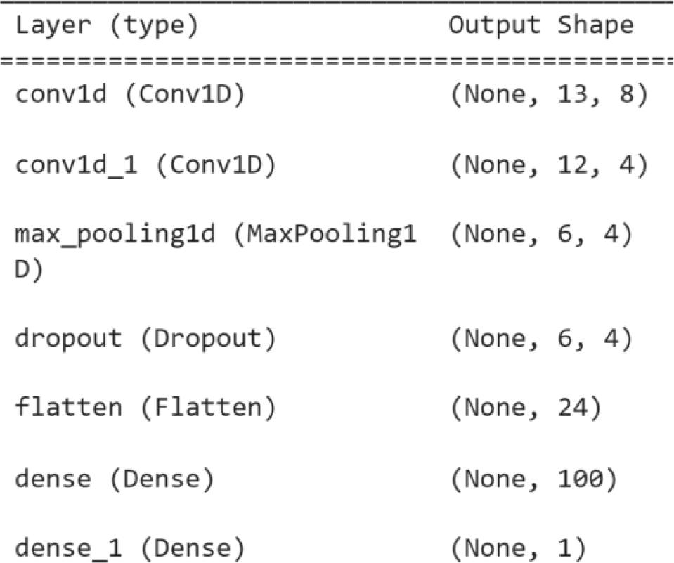
Model architecture
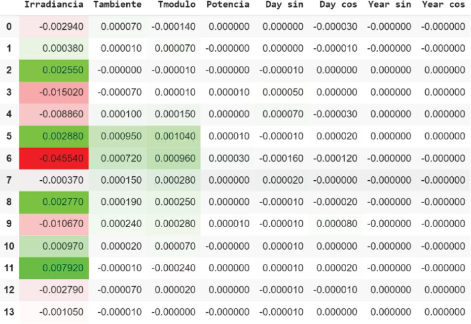
To represent the explanations, when using twodimensional tensors (14, 8), it was decided to use tables to represent the importance of each input characteristic.
Green represents a positive importance (Positive Contribution) to the prediction.
Red represents a negative importance (Negative Contribution) for the prediction.
With LIME it is shown how each characteristic contributes to the prediction, where it can be seen that the characteristic that most contributes to the prediction is the “Iradiancia” in all the days that are looked back, and in the same way we can see that the variable “Tmodulo” has no positive contributions to the prediction. The Figure 2 shows the results by using LIME explanation.
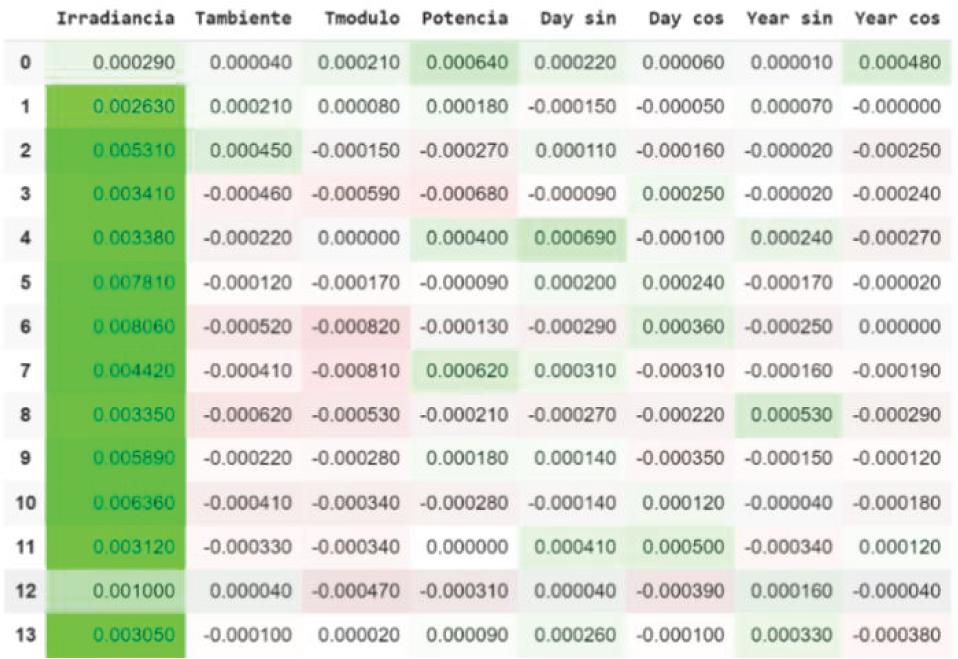
Explanation obtained with LIME
SHAP (Figure 3) yields results very similar to those obtained with LIME. In both cases, “Irradian-cia” across the entire look-back window is the feature that contributes most to the prediction, whereas “Tmodulo” shows no positive contribution.
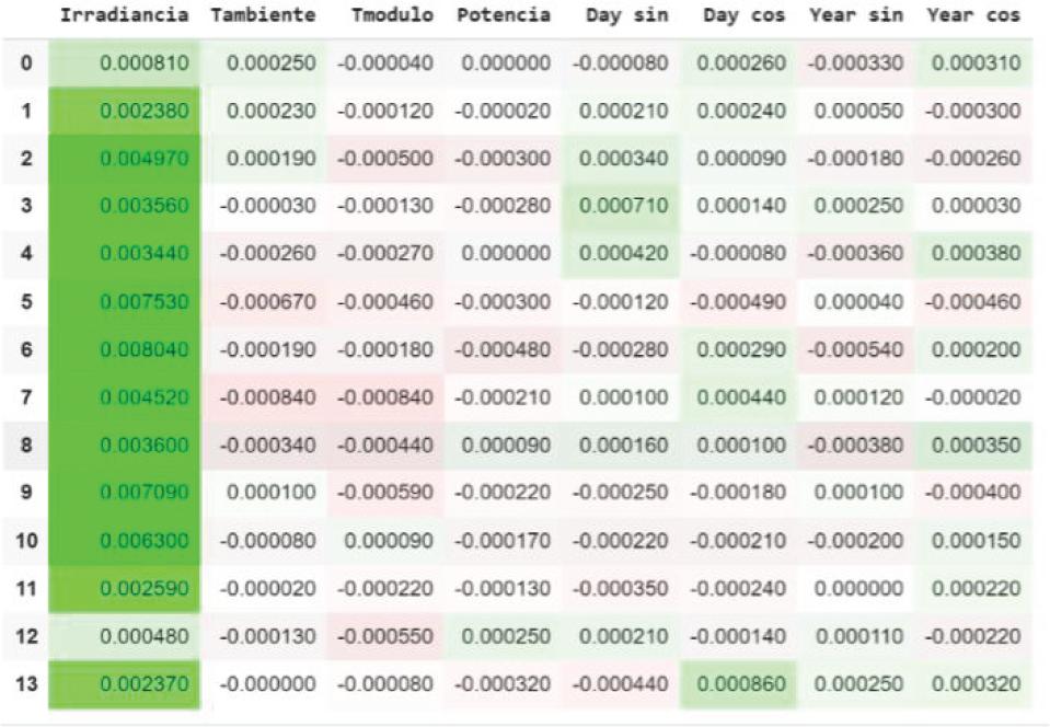
Explanation obtained with SHAP
Integrated Gradient offers a different explanation from that obtained by the LIME and SHAP methods (Figure 4), but on the contrary, similar to that obtained with the Time Series Saliency, where “Irradiancia” is a variable that greatly influences the prediction, but depending on the day in the past, can have a negative contribution to the prediction. It should be noted that for this method the variable “Tmodulo” has the greatest importance for prediction.
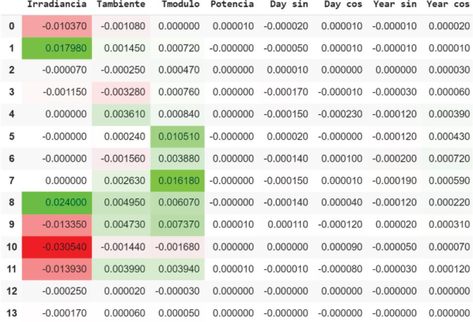
Explanation obtained with Integrated Gradients
This method obtained an explanation that is similar to each of the previous methods, since once again we can see that the variable “Irradiancia” has greater importance than the rest of the variables, depending on the day. In the past, it presents negative contributions, closely resembling the previous methods explained. It should be noted that in this case, like LIME and SHAP, the rest of the variables do not have significance except “Tmodulo” which, similar to Integrated Gradient, has a positive importance in the explanation. This is shown in Figure 5.
Explanation obtained with Saliency Maps
To compare the explanations obtained with these methods, the forms of evaluation of explanations mentioned in section 5 are used.
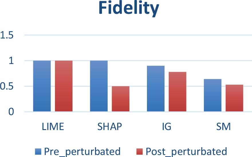
Fidelity values of methods
The comparison of the fidelity of the LIME, SHAP, Integrated Gradients and Time Series Saliency methods before and after perturbations, highlights the stability of LIME against changes in the data maintaining a perfect fidelity of 1.0, indicating that this method offers consistent interpretations and is robust to disturbances.
On the other hand, SHAP experiences a substantial drop in fidelity from 1.0 to 0.55 upon perturbations, highlighting its sensitivity to changes in the data. Such SHAP variability could be useful for exploring how different conditions affect the model, although this may imply reduced reliability in scenarios where consistency is required.
Finally, the Integrated Gradient and Time Series Saliency methods present a medium stability in the face of changes in the data, experiencing a drop of 1.2 and 1.1 respectively.
The results suggest that, depending on the need for consistency in interpretations, LIME could be preferred over the rest of the methods in contexts where interpretive stability is crucial, although Integrated Gradient and Time Series Saliency can also be considered.
These minimum continuity values offer crucial insight into the reliability of explanation methods when faced with variations in the data.
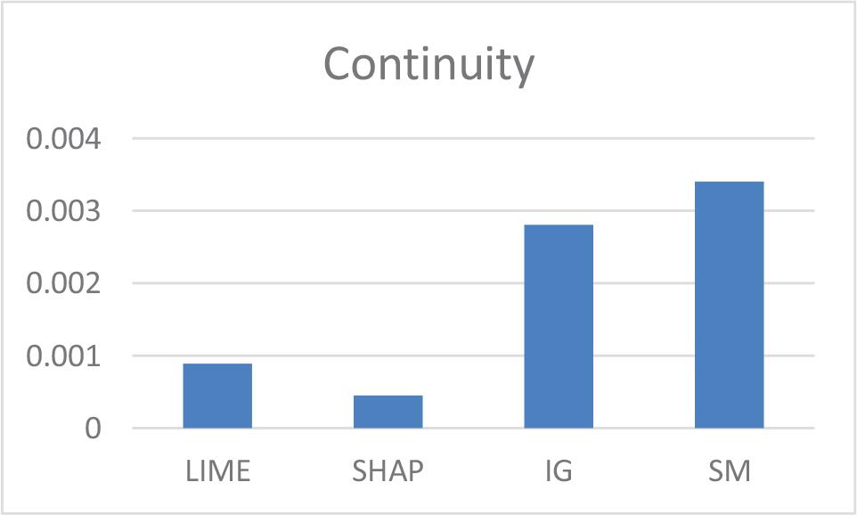
Method Continuity Values
LIME proved to be the most robust and consistent method, maintaining perfect fidelity in the face of changes in the data. It is suitable when stability is crucial.
SHAP had the greatest variability in explanations, although it could be useful to explore how different conditions affect the model.
Integrated Gradients and Time Series Saliency showed intermediate stability.
In terms of continuity, SHAP was the method with the least variability in explanations, followed by LIME.
Quantitative evaluation is important to objectively compare the quality of the generated explanations and select the most appropriate method according to the requirements.