Partitioning of Complex Discrete Models for Highly Scalable Simulations

Spectral graph partitioning methods are based on the selection of a subset of vertices that divides the graph into disjointed components. Such divisions seek to is to choose the smallest subset and divide the graph into subsets with an equal or close to equal number of vertices. Those methods use the Laplacian matrix representation of a graph. There many approaches for this method; for example, [11] presents the method using an algebraic approach to computing vertex separators, while [12] describes the spectral nested dissection algorithm (SND). These two algorithms use knowledge of the spectral properties of the Laplacian matrix to calculate the vertex separators in the graph, which determines the partitioning of the graph. These methods are expensive, however, due to the computation of the Fiedler vector, which selection criteria for vertices for the partitions. In [1], an attempt to shorten the execution time is proposed - the Fiedler vector is calculated using the multilevel spectral bisection algorithm (MSB). However, such improvements are still very computationally demanding.

The recursive methods are generally simpler to implement, but do not work so well for more complex problems, mainly due to the greedy nature of these algorithms. The method presented in [2] assumes division of the graph into a number of areas equal to a power of two. This method can also divide the graph according to the computational capabilities of the individual processor cores. However, the underlying idea of dividing the graph into smaller and smaller parts precludes the algorithm from taking indivisible parts into account without significantly altering the idea underlying it.

Geometric methods use the geometric data layout of the graph for optimal partitioning. Their main advantage of these methods is their relatively short execution time, but they achieve lower-quality division results than the spectral methods. One of the best uses this method is presented in [6], where the authors describe an effective way of partitioning unstructured graph environment, which is useful for the FEMs (finite element methods) and FDMs (finite difference methods). This approach uses the geometry of a given graph to find a partitioning in linear time. They can be applied to graphs representing two- and three-dimensional grids. A characteristic feature of geometric methods, resulting from their random nature, is the need to execute the algorithm anywhere from 5 to 50 times to obtain results comparable with spectral methods, while still maintaining a shorter computing time. Geometric methods are applicable only when the coordinates of all vertices in the graph are available. For many problems (linear programming, VLSI), such coordinates are not available, limiting the applicability of this method. There are also algorithms that are able to calculate coordinates for graph vertices using spectral methods [3], but they significantly increase computing time.

A characteristic feature of the multilevel graph partitioning approach is the reduction of the graph size by combining the vertices and edges and dividing the reduced graph into partitions. The last phase restores the initial graph while preserving the obtained partitioning. The graph is often reduced until the number of vertices reaches the desired number of partitions [7]. The phase of restoring the graph to its initial size is accompanied by an algorithm aimed at improving the division [4]. Operating on a reduced graph has lower computational costs than other approaches. The methods in this class reduce the length of the boundary between partitions while maintaining the proportional sizes of the areas. Such methods were initially intended to reduce partitioning time at the expense of quality. The multilevel partitioning method is described in more detail in Section 3.

Recent research suggests that multilevel methods yield better results than spectral methods. Libraries such as Party [7], Metis [5], Jostle [17] are based on a multilevel partitioning scheme and currently give the best results in terms of partitioning quality.

The authors of [7] compared these algorithms by partitioning a 100x100 grid area into 16 partitions, as demonstrated in Fig.1. All of these methods reduce the graph; however, only Jostle and Party reduce the graph until they get the number of vertices equal to the required number of partitions. By comparing many different examples of grid partitioning problems, Party seems to outperform other algorithms, as shown in Fig.1c. Moreover, Jostle has problems with partitioning the grid into appropriate areas. It can be observed that elongated, irregular partitions increase the edge-cut, even though boundaries between adjacent partitions are relatively straight.

Figure 1.

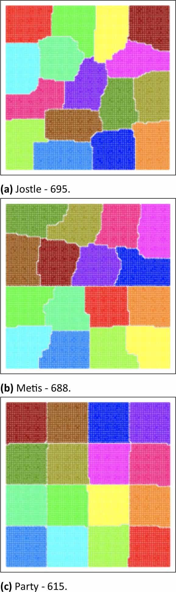
Partitioning a 100x100 grid into 16 areas; the edge-cut value is shown in the caption for each method. [7]

None of the above-mentioned methods take the problem of indivisible areas and areas excluded from the calculations unused areas into account.

The multilevel graph partitioning methods [7] are the most promising and give the highest-quality results. As shown in Fig.1, Party yielded the best results and as such, the presently proposed solution improves upon it. The main goal is to propose a solution that will be able to support both indivisible areas and excluded areas, while providing high-quality graph partitioning.

An initial graph is built from an image. Each pixel on the image represents a vertex. Colors represent different graph area types; yellow areas are the indivisible areas, while red areas are the excluded areas. Normal areas are white. In the graph that is created, the normal area contains vertices with a weight of 1, while excluded areas are either removed from the graph or contain vertices with a weight of 0. Every indivisible area is mapped into a single vertex with a weight equal to the sum of the weights of the vertices in that area (Fig.2). Thus, very time a set of edges is replaced by a single edge, the weight of the single edge is a sum of the replaced vertices’ weights.

Figure 2.

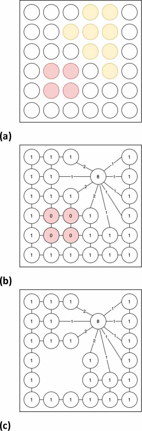
Excluded areas are either removed from the graph (c), or their weights are set to 0 (b).

This condition allows for balanced vertex matching, avoiding vertices with very high weights along with vertices with relatively small weights. The weight of the new vertex is the sum of the weights of the matched vertices.

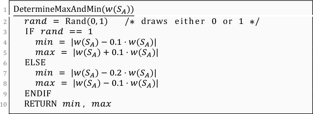
The first change introduced by us to the LAM algorithm is an extended condition for matching vertex a with vertex b (3):

To create a smaller graph, a heuristic of a matching algorithm is introduced. In our case, it is the LAM [13] matching algorithm, which is executed until the number of vertices is equal to the desired number of partitions. It starts from a randomly chosen edge and checks adjacent edges. As long as it manages to find adjacent edges with a higher weight, the algorithm switches onto them and repeats the procedure until it finds the edge with the highest weight. Vertices at the end of this edge will be matched only if they satisfy a certain condition; in the Party [7] implementation, two vertices, a and b, with weights w_a and w_b, could be matched only if their combined weight did not exceed double the lowest weight (w_lowest) plus the heaviest weight (w_highest) that occured in the whole graph (Equation 1). 1wa+wb≤whighest+2·wlowest{w_a} + {w_b} \le {w_{highest}} + 2\;\cdot\;{w_{lowest}} 2discount=tT·whighestwlowest+1·log(num_of_partitions)+1discount = {t \over {T\;\cdot\;{{{w_{highest}}} \over {{w_{lowest}} + 1}}\;\cdot\;\log (num\_of\_partitions) + 1}} 3wa+wb≤discount·(whighest+2·wlowest){w_a} + {w_b} \le {\rm{ }}discount{\rm{ }}\cdot\;\left( {{w_{highest}} + 2\;\cdot\;{w_{lowest}}} \right)

If discount > 1, it is assigned a value of 1. T is the expected number of LAM algorithm executions. It is counted as the number of times the number of graph vertices has to be divided by 2 to get a number of vertices that is less or equal to the number of partitions required to achieve it. t is the current number of LAM algorithm executions. The condition established by authors of the Party library assumes a balanced formation for the vertices’ matchings from the very beginning of the algorithm execution.

In our case, however, this assumption is disturbed by vertices made from indivisible areas, which may have very high weights at the beginning of the algorithm execution. As a result, without our modification, the algorithm gives poor-quality results (Fig.3).

Figure 3.

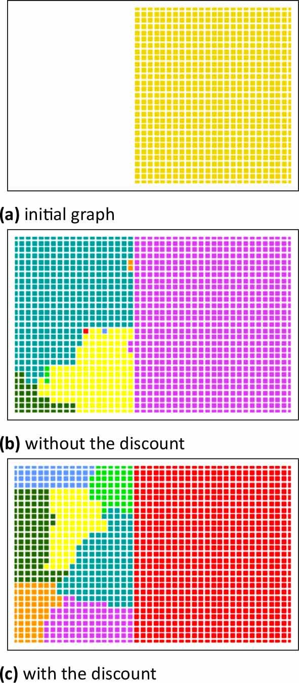
Effects of the partitioning with and without the discount.

Adding the discount to the matching conditions enhances the condition and creates more balanced vertex matchings, especially in the initial algorithm executions. The later the iteration, the more similar it becomes to the original condition.

The other modification made to the LAM algorithm is the removal of the R set, which contains edges that are about to be removed. It is not useful for the graph shrinking application, so its maintenance can be skipped.

The second part of the graph partitioning algorithm is the refinement and restoration phase. It takes as an argument a shrunken graph and iteratively restores it to the initial size. After the graph is about 90% restored, the refinement procedure starts alongside the restoration, which aims to reduce the edgecut and balance the sizes of the partitions. For the refinement phase, the algorithm based on the Helpful Set heuristic [15] was used.

The implemented Helpful Set heuristics (Code 1) start from the initial partitioning and reduces the edge-cut using locally performed changes.

Code 1.

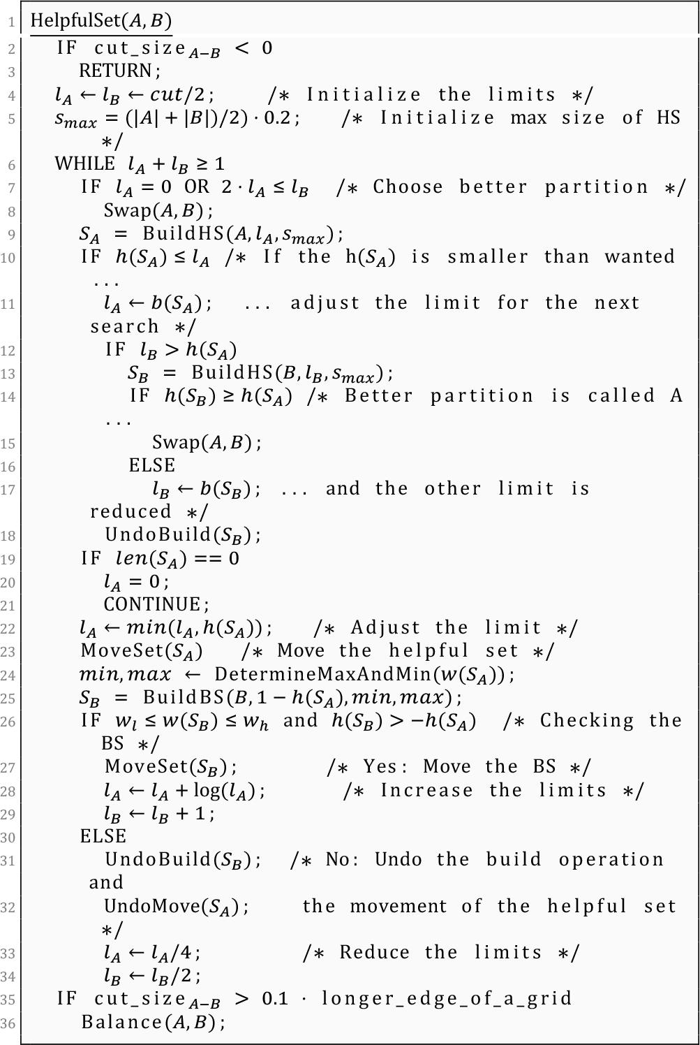
Modified Helpful-Set algorithm.

As an example, let us take partitions V₁ and V₂. It starts from the initial set k-helpful, which is a subset of V₁ or V₂ that reduces the edge-cut by k if it is moved to the other partition. Let us assume that k-helpful was found in V₁. Then it is moved to V₂. In the next step, the algorithm starts to look for a balancing set in the V₂ partition. This set has to balance the partitions (reducing sizes to be similar to the initial ones), and it can increase the edge-cut maximally by (k – 1) edges. If a balancing set is found, then it is moved to V₁. This results in an edge-cut decrease of at least 1. Vertices that build a helpful set and a balancing set are added greedily and are stored in a sorted priority queue according to their value. The most important part of the algorithm is to figure out the l helpfulness values for the sets. If l is too small, then good sets cannot be found; if l is too big, then the execution time is longer, but the found sets are not necessarily better. To compute l value, Party uses an adaptive limitation technique. It contains two l limits - a separate one for each of the sets.

Several modifications have been introduced to the original algorithm in order to adjust it for the considered requirements.

The first concerns the initialization of s_max. Originally its size was set to 128, while in the proposed method it is dependent on the sizes of the partitions (line 5). Used for this purpose, the 0.2 factor could be changed - but, according to the experiments, it should not be more than 0.4, to prevent the helpful set from getting too big. The condition for the WHILE loop was weakened from ≥ 0 to ≥ 1 to decrease number of the algorithm executions. The additional repetitions did not improve the partitioning, but worsen execution time. In Party’s solution, during the search, the helpfulness of the helpful set is > –d/2, and its weight cannot exceed s_max. d is an average vertex’s degree in the graph. In our case, d = 4. This rule happened not to work, however. The algorithm is greedy and often builds sets, which fulfilled the s_max condition and with –2 ≤ helpfulness ≤ 0. But when, in the original code, it was checked whether helpfulness < 0, and if true, the helpful set search had to start once again. Because of this, the algorithm was running unsuccessfully for multiple times. The solution to this issue was a change in the instruction for the condition for the size of the S_a (line 19), allowing for the building of helpful sets with a helpful value ≥ 0 (line 9 and 13). The helpful-set algorithm has a mechanism to build a helpful set from a more promising partition (line 7). After the helpful set is found - which might happen after further adjustments to the l value - the balancing procedure starts, and a [min, max] range is computed. This is the minimum and a maximum weight of the balancing set. max is a little bigger than size of the helpful set and min is a little smaller. During the experiments, the algorithm was usually reaching max size - and for some reason, for each pair of refined partitions, the same one was usually chosen to build the helpful set from; the same was true for balancing set. As a result, one partition was always growing at the expense of the other. As a result, the following change to computing the min and max values was introduced:

Code 2.

Modified min and max computing.

If a balancing set’s weight is in the range, it is moved to the other partition. The next modification was the condition for executing the Balance procedure, which prevents the formation of scattered areas. The Balance procedure greedily chooses vertices with the highest helpfulness. These are always vertices from a bigger partition. It does not move the whole weight difference between the partitions; instead on each execution, it moves only a percentage of this difference. In our case, it was around 10% of the weight difference.Making local refinements can cause scattered partitions to appear. A scattered partition is a partition that is divided into unconnected sub-areas. This can be caused by indivisible areas, which are usually big chunks of a graph that can be moved in just one step of the refinement algorithm. A simple solution is to find scattered partitions; identify the main, biggest subarea; and join the other parts with their adjacent partitions. This procedure is executed after each refinement.

Considering modern parallel hardware architectures - which are composed of multiple nodes, each equipped with multiple cores - requires taking into account differences in local and remote communication. Partitioning of a grid for parallel processing on m nodes with k cores each should provide m subgrids, each divided into k partitions. The simple approach of dividing the grid into m parts first and then splitting each part later cannot be used here because of the indivisible parts of the grid; a single indivisible part might become one of the m parts, preventing its further division it into k parts. Therefore, it is proposed to merge the m · k division into m parts instead.

This part is handled by the LAM weighted matching with an additional greedy algorithm. First, after the partitioning into m · k parts, the graph is reduced to m vertices using the LAM matching algorithm. After the reduction, each vertex is assigned to a new partition. Next, the graph is restored to m· k partitions, but the m partitions yielded by LAM are kept. At this point, if not all of the m partitions have the same amount of subpartitions, the greedy method is used: first, the adjacent partitions are balanced. Next, if there are no more imbalanced adjacent partitions, but there are still some imbalances, the algorithm chooses the two partitions with the highest and lowest number of vertices and balances them greedily. This process is repeated until all the partitions have a proper size.

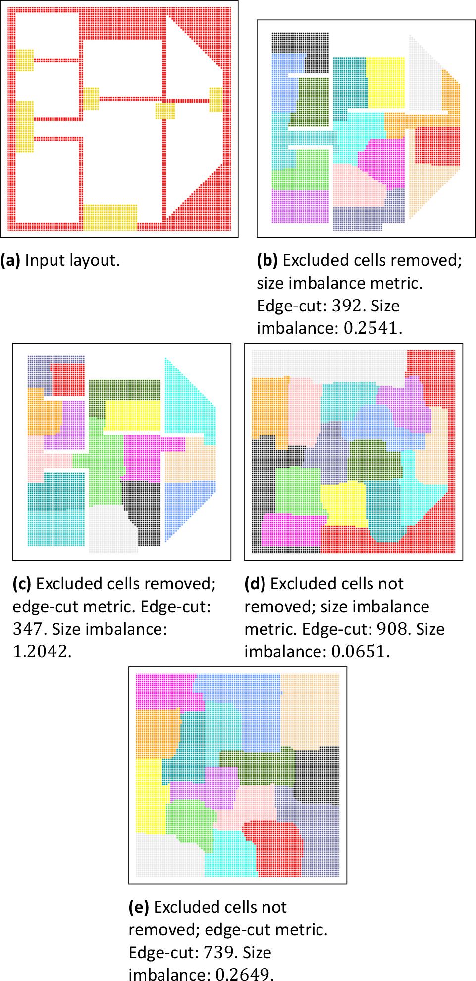
In the first experiment, the grid is a building floor plan, with several rooms connected via hallways (see Fig.4a). The grid contains both excluded areas and indivisible areas, which are represented as red and yellow pixels, respectively. Walls and the area outside of the building are marked as excluded areas, while doorways are marked as indivisible. The size of the grid is 100 × 100 cells, and divided into 16 partitions.

Figure 4.

Results of a building floor - plan partitioning.

The experiment was executed in four variants, determined by two parameters:

• –

  Excluded areas were either assigned a zero weight or removed from the graph.

• –

  The metric used to determine the best result was either edge-cut or size imbalance.

Fig.4 shows the input and the results of the partitioning. In each case, the input constraints were preserved, i.e., the excluded area did not cause large imbalances in area sizes, and indivisible areas remained undivided.

It is easy to observe that removing the excluded cells yielded better edge-cut metric values (see Fig.4b and Fig.4c). However, it is also important to notice that a lot of connections are removed from the graph, which significantly reduces the ability of different areas to be connected. At the same time, the borders that would touch excluded areas on one or both sides might have no communication in the simulation system, as those areas do not take active part in the simulation by definition. Another interesting piece of information is that preserving the excluded cells yielded much better size - imbalance metric values (see Fig.4d and Fig.4e). This might be caused by the ability to connect remote areas via a patch of zero-weight cells that do not cause the area to stop expanding.

In opposition to the usual LAM algorithm behavior, which tends to yield partitions with smaller perimeter to area ratios, the use of zero-weight cells caused more elongated shapes to emerge. One consequence is that a non-excluded area taking part in the simulation might become disconnected within a single partition - this is easiest to observe with the red partition in Fig.4d.

The conclusions from this experiment are evidence in favor of removing the excluded areas from the graph entirely. It leads to better division of the actual, used parts of the grid.

In the second experiment, the given partitioning into m · k areas was partitioned into m areas. This operation is strictly connected to the underlying idea of partitioning the grid for paralellization of computations. In the scenario in which the simulation will be executed using m nodes with k cores each, the first step creates the partitions for each core, while this step assigns them to the nodes.

This experiment was performed using two example scenarios. The first one is a synthetic example, in which a grid of size 100× 100 was already partitioned into 24 areas. The experiment consists of two executions of partitioning those areas into 6 and 4 larger areas (thus m = 6, k = 4 and m = 4, k = 6). Fig.5 shows the results of this partitioning. The input partitioning (see Fig.5a) has a better size-imbalance metric value, but a much worse edge-cut metric value than both outputs. This is to be expected, as division of any area creates a new border, and thus the edge-cut should be larger for any partitioning with more areas. At the same time, any inequality in area sizes might be magnified by combining them into larger groups. Both outputs show some disconnection in the final partitions, which contributes towards larger edge-cut, but the metric value is improved in both cases. As the interpretation of this metric for merged output is the amount of inter-node communication, these results are very promising.

Figure 5.

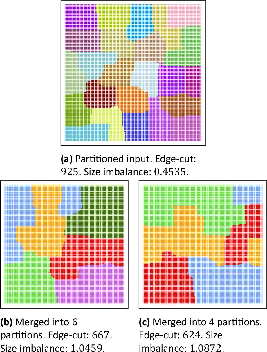
Synthetic example of partitioning.

The second scenario is a building floor plan, based on the same layout as shown in the first experiment (see Fig.4a). The size of the grid is 100 × 100, m = 4, k = 4. Fig.6 shows the results of this experiment. The most important quality of the resulting division is that it consists of 4 areas of almost identical sizes, which can be further divided into 16 smaller areas, enforcing the rules of the excluded and indivisible cells in both cases. Not all areas are continuous - the red area in Fig.6b is divided into three parts. However, it can be easily shown that there is no partitioning of the input that avoids fragmentation in the resulting partitions. The red area in Fig.6a isolates two branches of the floor plan - one containing three partitions, and the other containing two. Merging the red area with any of the groups will leave the other unable to connect to sufficient number of areas to form a 4-area group.

Figure 6.

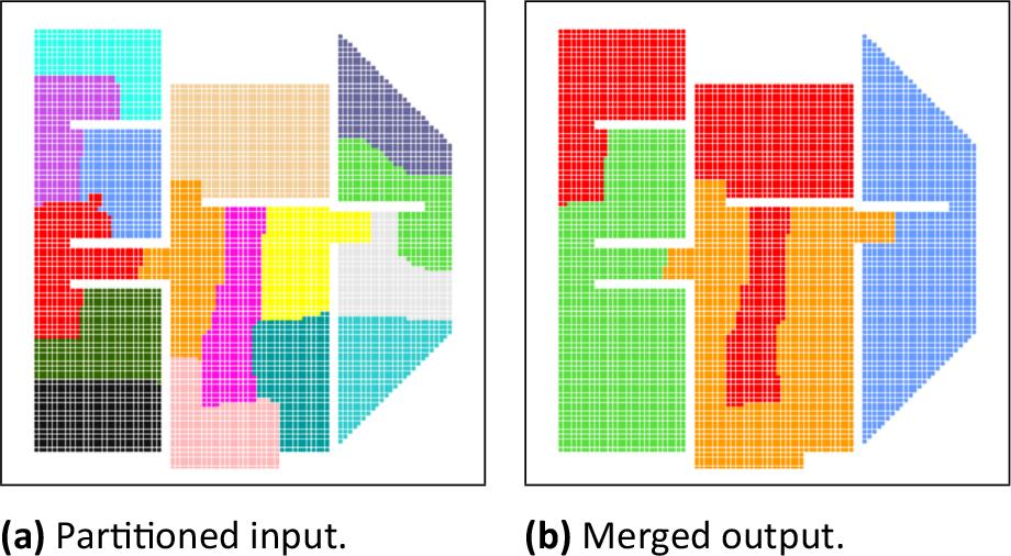
Plan of building floor example of partitioning.

Edge-cut: 200. Size imbalance: 1.6641.