
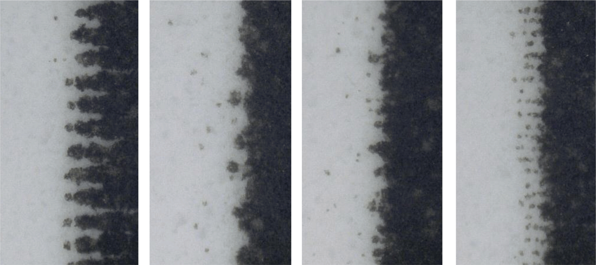
Figure 1
Differences in the spatial distribution of satellite droplets from four inkjet printers of different type and model.
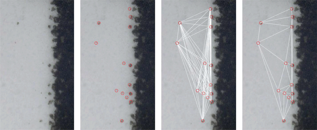
Figure 2
From left to right: (1) Satellite droplets and border of a printed character, (2) manually marked satellites, (3) complete graph connecting every point with each other, (4) Delaunay triangulation.
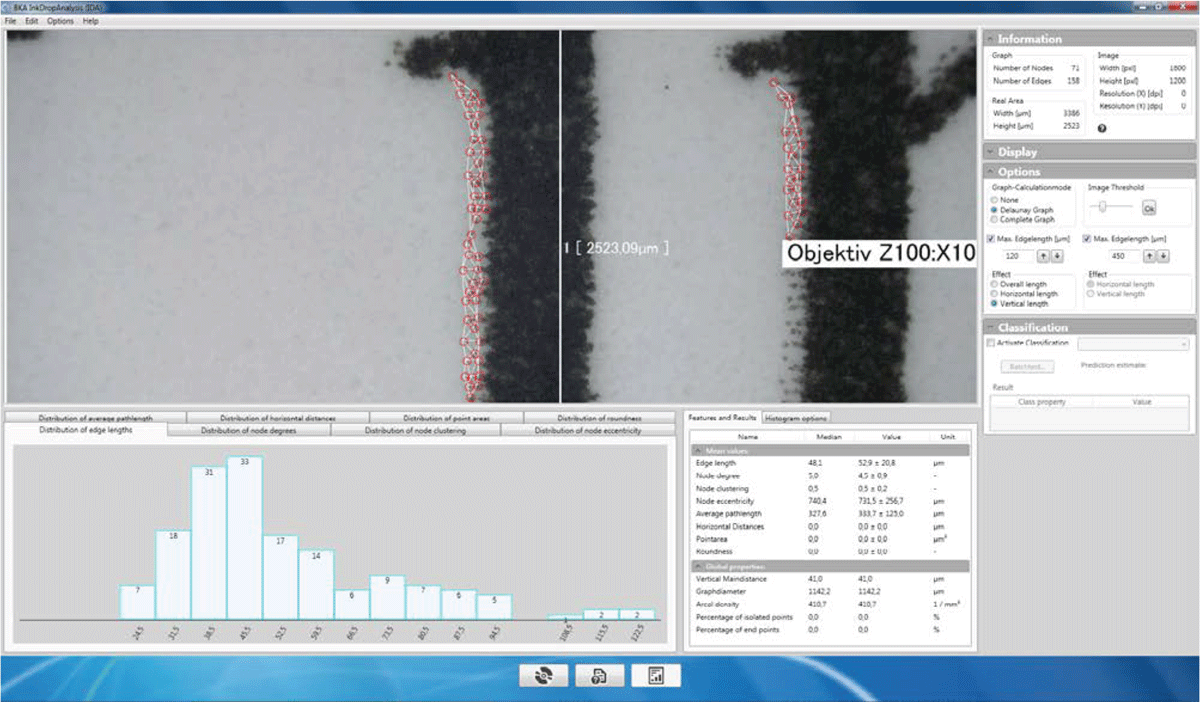
Figure 3
Screenshot of the software implemented and used in the experiments: The big area on the top-left shows a picture of the region of interest of the printed document together with marked satellites (red circles) and a Delaunay triangulation restricted by two orthogonal thresholds (white lines). On the bottom-left each tab contains a distribution histogram for a statistical property of the graph (histogram of the edge lengths on this screenshot). The table on the bottom-right contains the median, average and standard deviation of the corresponding histogram.
Table 1
Topological attributes and global label attributes of the graph used to build a feature vector.
| Name | Description |
|---|---|
| Edge length | Average (Avg.) and standard deviation (std. dev.) of the length of all edges. |
| Degree | See13 |
| Clustering coefficient | See13 |
| Effective eccentricity | See13 – Shortest paths are calculated using15. |
| Average Pathlength | For each node the average of the shortest paths to each other node is calculated. The distribution of these averages yields Avg. and std. dev. |
| Vertical main frequency | The most prominent value of all vertical distances for a profile which should be related to nozzle distance and thus to vertical resolution. |
| Graph diameter | See13 |
| Areal density | Number of nodes per area. |
| Isolated Points | See13 |
| End Points | See13 |
Table 2
The inkjet printers used in the experiments. For each type in this table there have been three individual printers making a total of 12 printers.
| Make | Model |
|---|---|
| Brother | MFC-J825DW |
| Canon | Pixma MG 5350 |
| HP | Photosmart 6510 |
| Kodak | Hero 7.1 |
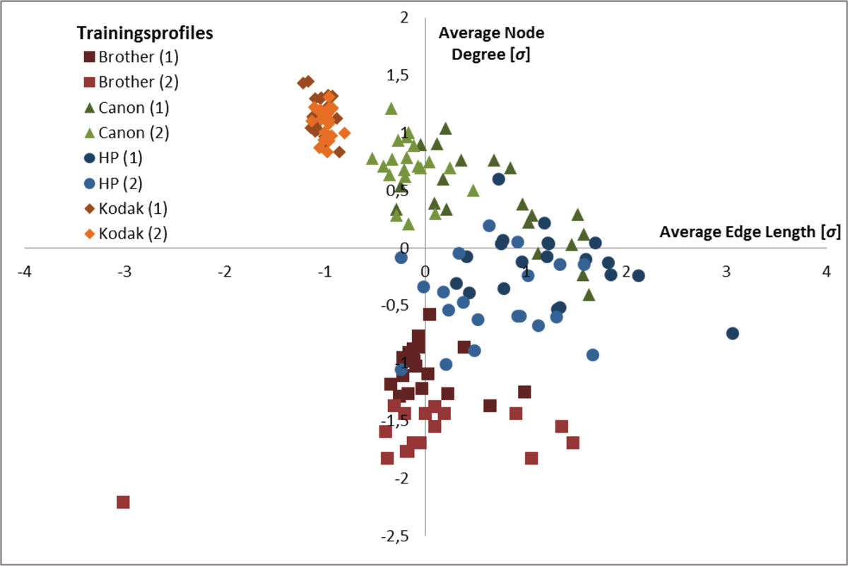
Figure 4
Average edge length vs average node degree taken from the feature vectors of the trainingprofiles.
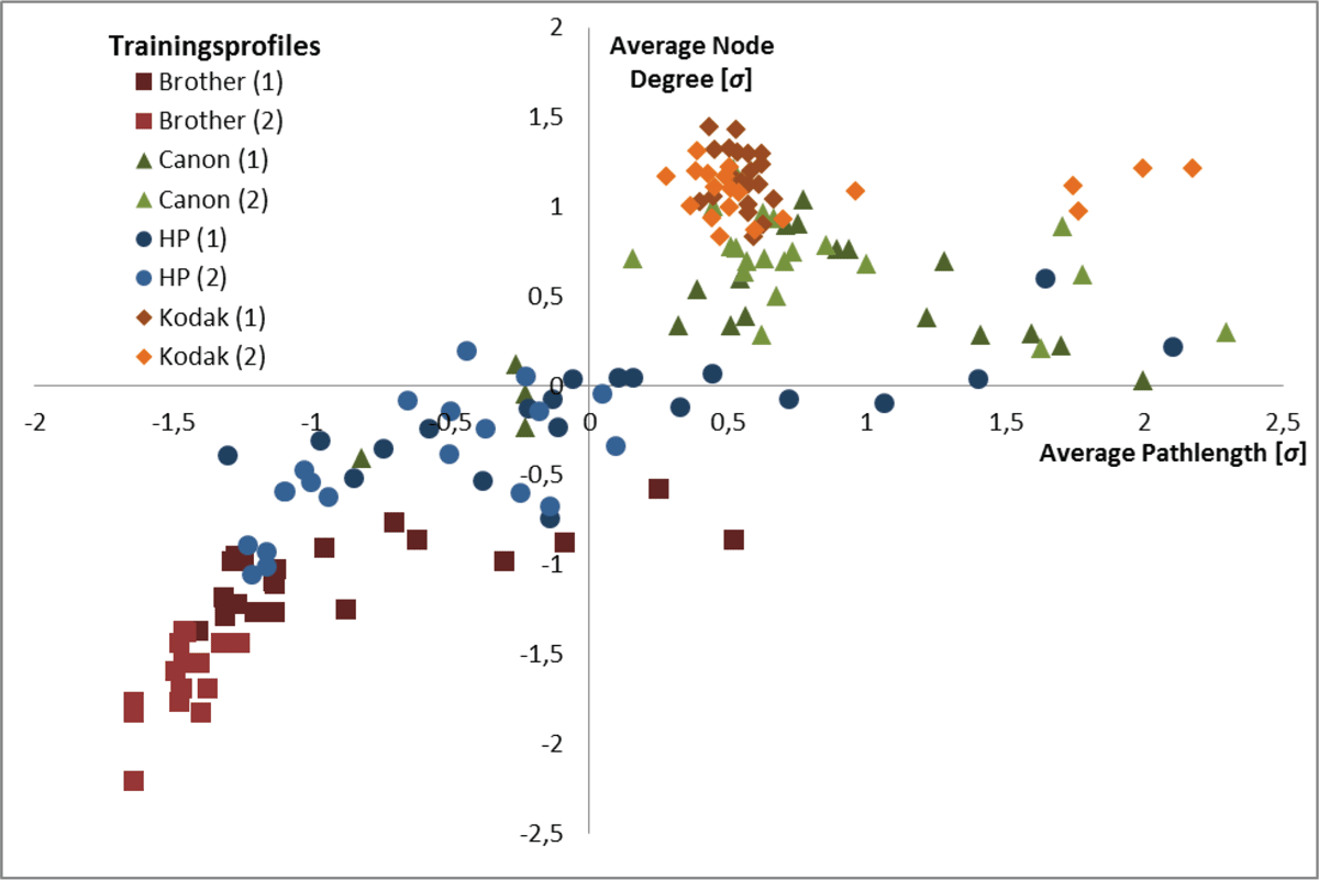
Figure 5
Average pathlength vs average node degree taken from the feature vectors of the trainingprofiles.
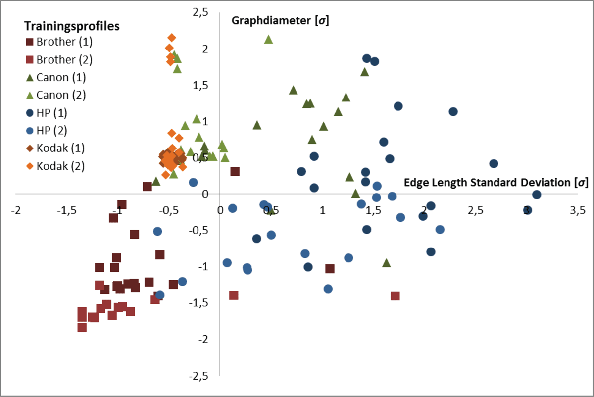
Figure 6
Edge Length std. dev. plotted against Graphdiameter taken from the feature vectors of the trainingprofiles.
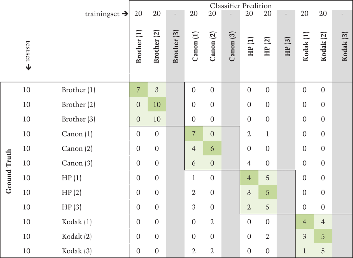
Table 3
Results of the classification of the test set (per device).
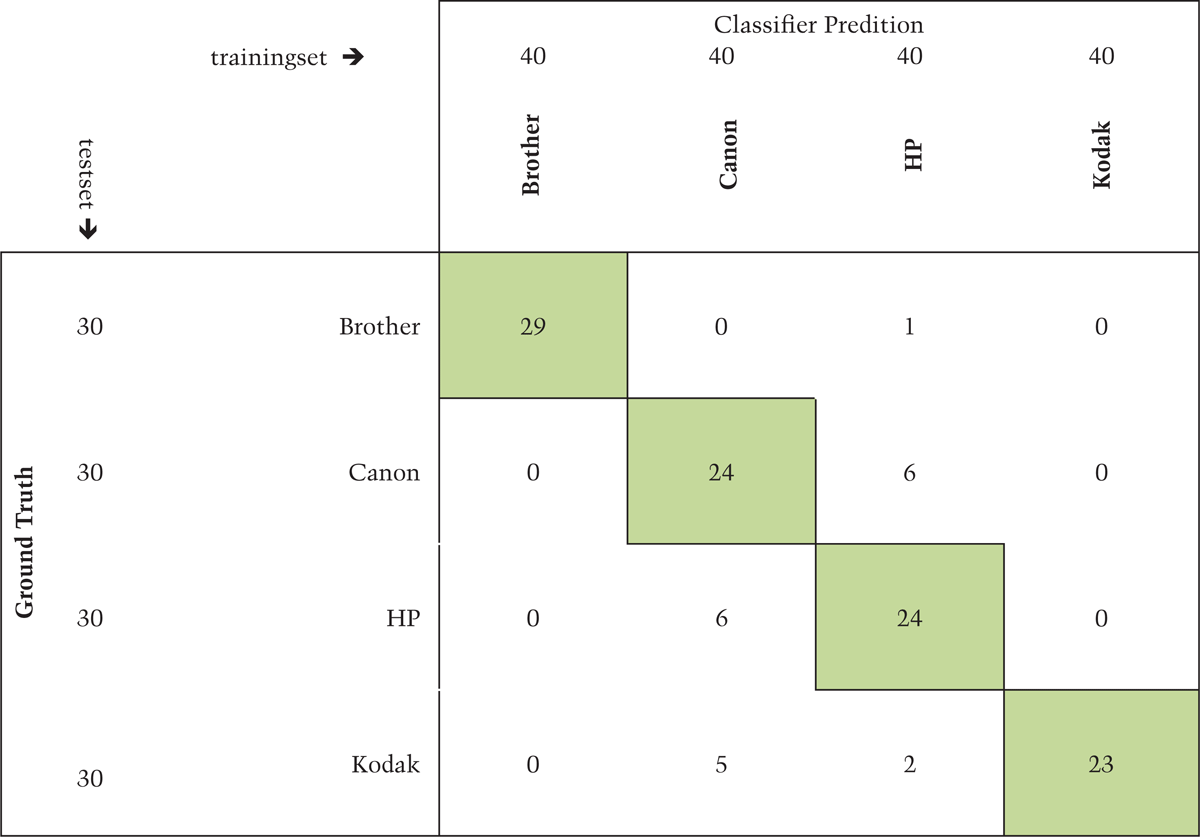
Table 4
Results of the classification of the test set (per manufacturer).