
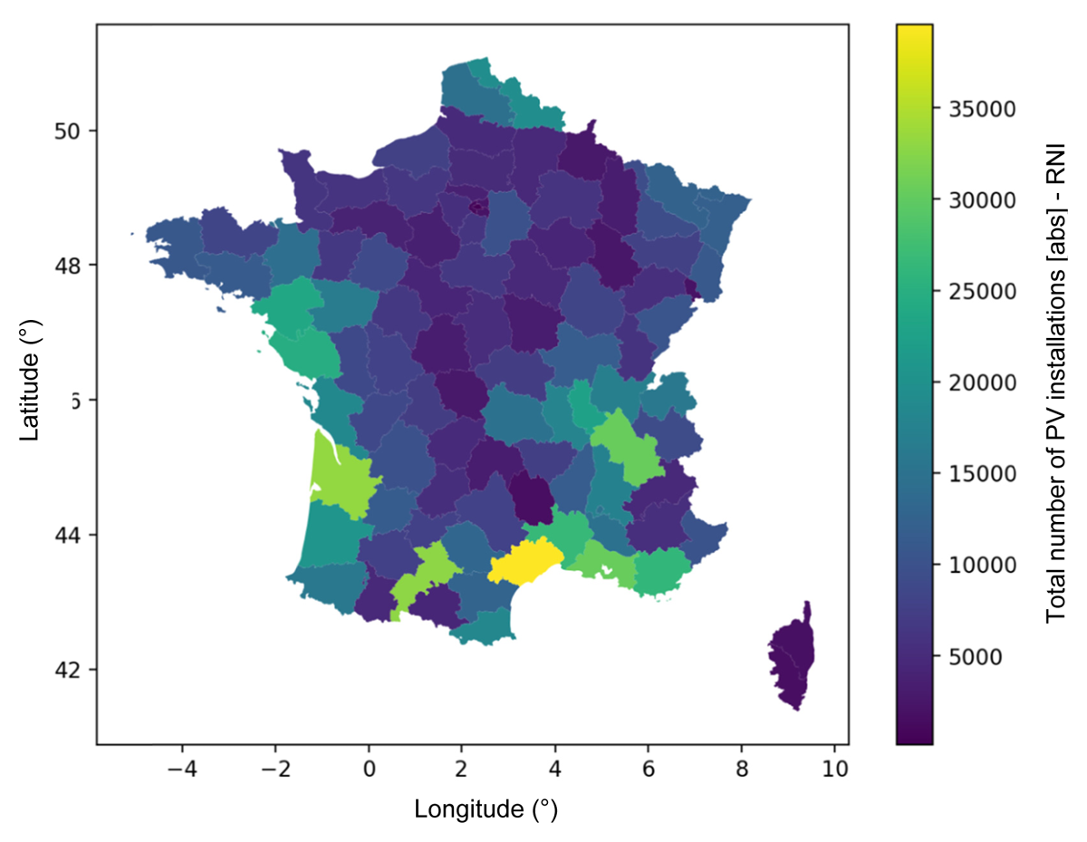
Figure 1
Map of the French department with the total number of PV installations below 36 kWp (source RNI).
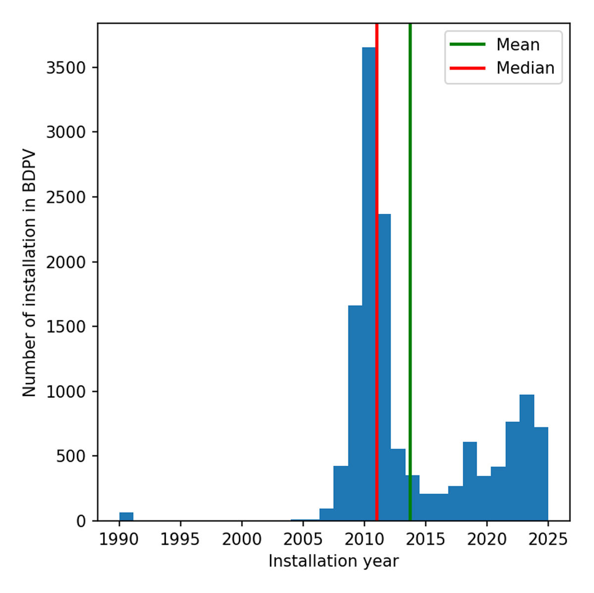
Figure 2
Distribution of the installation year of RPV installation in the BDPV.
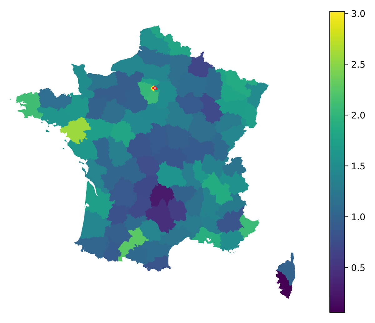
Figure 3
Ratio of installation in the BDPV dataset compared to the RNI.
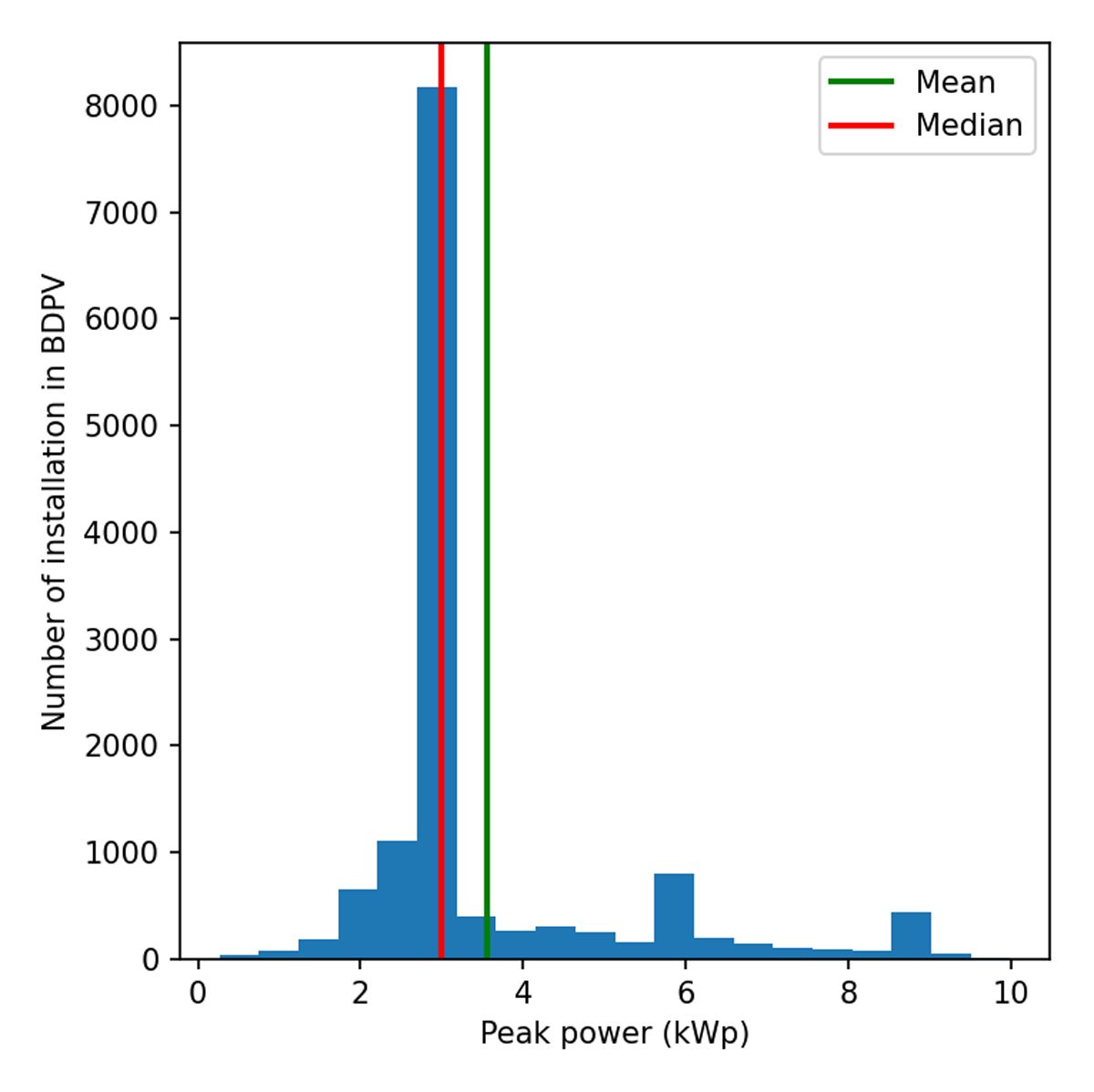
Figure 4
Distribution of peak power of RPV installations from the BDPV.
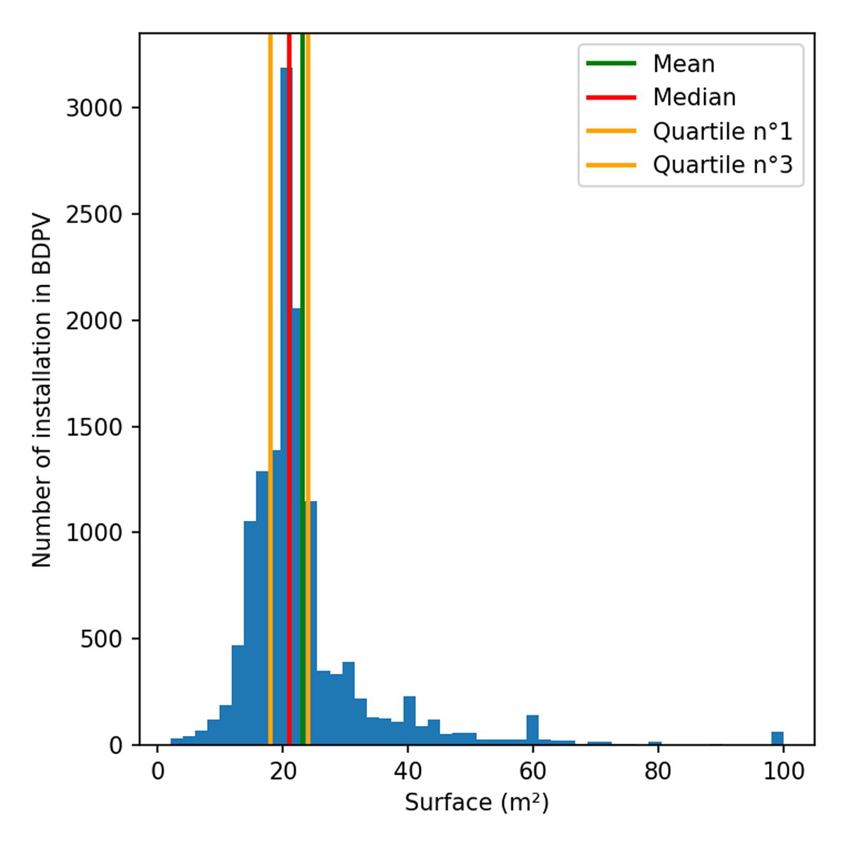
Figure 5
Distribution of the surface of RPV installations from BDPV.
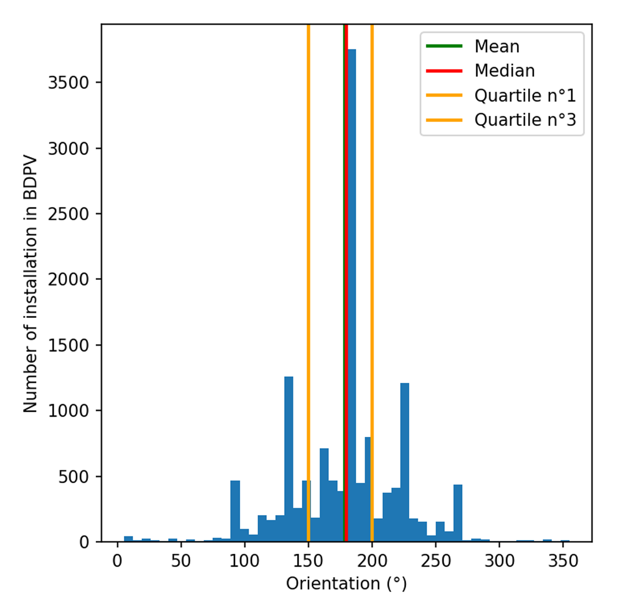
Figure 6
Distribution of orientation angle of RPV installations from BDPV (North = 0°, East = 90°, South = 180°, West = 270°).
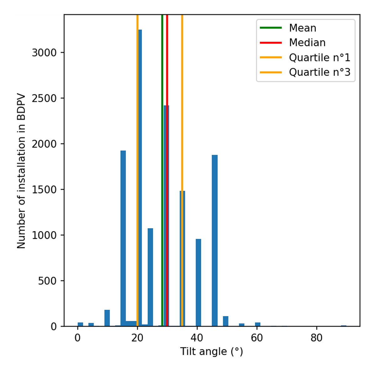
Figure 7
Distribution of tilt angle of RPV installations from BDPV.
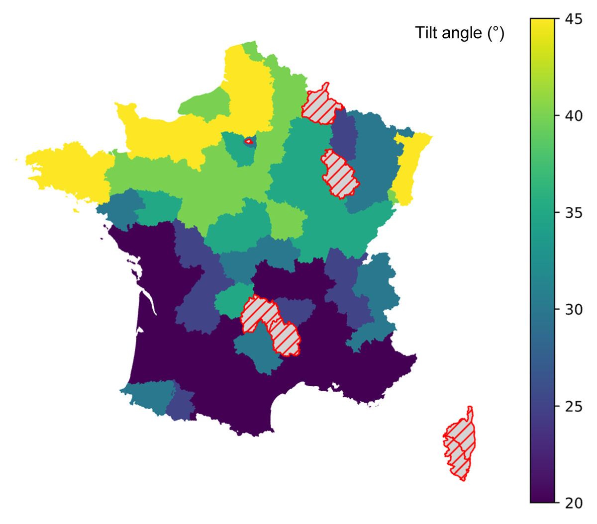
Figure 8
Map of the average tilt angle of RPV installation (°) per department from BDPV.
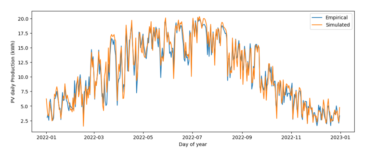
Figure 9
Average RPV daily production (kWh) for 1,000 installations from simulation (orange) and empirical measurement (blue) during the year 2022.
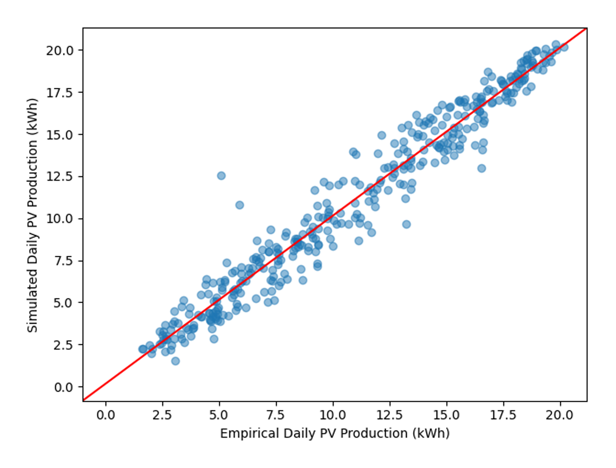
Figure 10
Average RPV daily production (kWh) for 1,000 installations from simulation as a function of empirical measurement value (kWh).
Table 1
Metrics between simulated and empirical RPV production. The first line is the metrics of the diversified load curve over 1,000 simulations. For the second line the metrics are computed across all individual simulations and then averaged.
| METRICS BETWEEN SIMULATED AND EMPIRICAL | R² | NMBE | CV(RMSE) |
|---|---|---|---|
| Metrics for the diversified production load curve | 0.95 | –0.01 | 0.11 |
| Average of the 1,000 individual metrics | 0.77 | 0.16 | 0.32 |
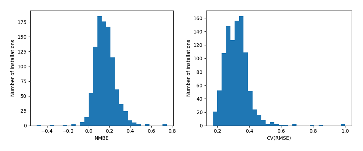
Figure 11
NMBE (left) and CV(RMSE) (right) distributions for the 1,000 simulated installations vs the empirical production from the BDPV. The left graph depicts the distribution of bias (NMBE) between simulation and empirical results of each of the 1,000 RPV installations.
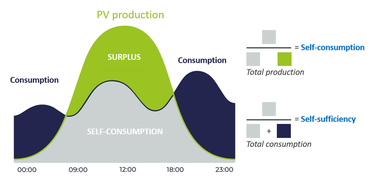
Figure 12
Schematic diagram of a PV production vs. consumption load curve and the associated metrics (self-consumption and self-sufficiency).
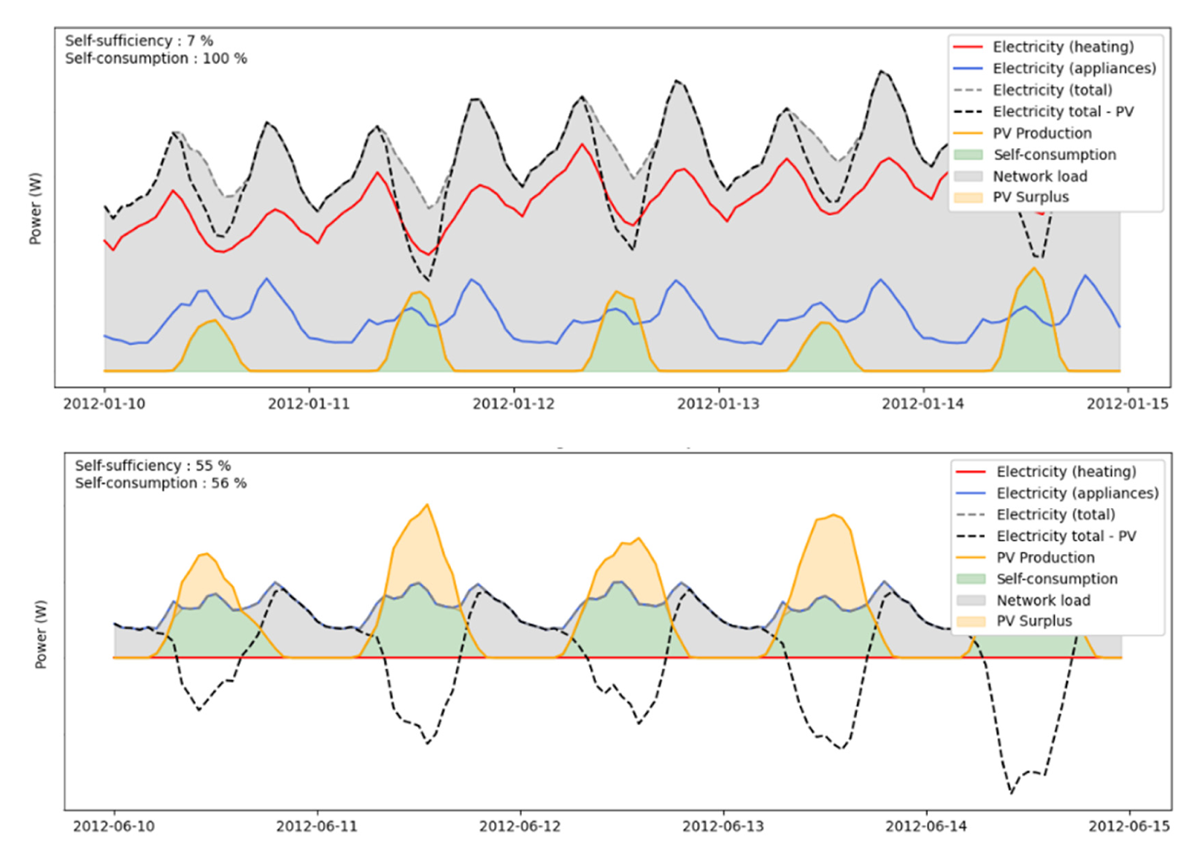
Figure 13
Simulated load curve for an average Joule-heated SFH of the stock. The Y-axis values have been removed for confidentiality reasons.
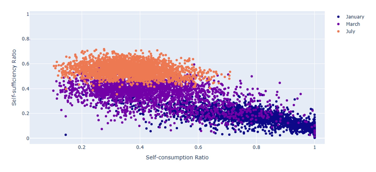
Figure 14
Self-sufficiency as a function of self-consumption. The metrics are computed for every day and every dwelling of the stock for the month of January (orange), March (purple) and July (orange).
Table 2
Average values of self-sufficiency and self-consumption per type of space heating (electric/non-electric) with a 3 kWp RPV installation.
| METRIC | MONTH | NON-ELECTRIC SPACE HEATING | ELECTRIC SPACE HEATING |
|---|---|---|---|
| Self-sufficiency | January | 20% | 10% |
| July | 55% | 55% | |
| Self-consumption | January | 73% | 89% |
| July | 37% | 36% |
Table 3
Average self-sufficiency and self-consumption by month for SFH with non-electric space heating as a function of the RPV peak power.
| METRIC | MONTH | RPV PEAK POWER PER DWELLING | |||
|---|---|---|---|---|---|
| 1 KWp | 3 KWp | 6 KWp | 9 KWp | ||
| Self-sufficiency | January | 10% | 20% | 26% | 29% |
| February | 21% | 32% | 37% | 39% | |
| March | 29% | 42% | 46% | 48% | |
| April | 31% | 47% | 53% | 56% | |
| May | 36% | 53% | 59% | 62% | |
| June | 36% | 54% | 61% | 64% | |
| July | 38% | 55% | 62% | 64% | |
| Self-consumption | January | 93% | 73% | 56% | 45% |
| February | 80% | 50% | 33% | 24% | |
| March | 72% | 39% | 23% | 16% | |
| April | 75% | 42% | 25% | 18% | |
| May | 72% | 39% | 23% | 16% | |
| June | 75% | 41% | 25% | 18% | |
| July | 72% | 37% | 21% | 15% | |