
Introduction
Context
Over the last decade, RPV panel installations surged significantly across Europe, reaching a total installed capacity of 215 GWp in 2024 – representing 61% of Europe’s total photovoltaic (PV) capacity (Ember, 2024). This expansion is largely driven by European decarbonisation targets and national energy policies that aim to accelerate the deployment of renewable energy sources. In France, the Programmation Pluriannuelle de l’Energie (PPE) (multiannual energy programming) sets ambitious targets for solar PV development, with the residential sector expected to play a significant role. In 2025, residential RPV-connected peak power reached 5 GW (ENEDIS, 2026). Until the early 2020’s, RPV individual production was sold entirely under feed-in tariff contracts at high prices, as a means to encourage RPV adoption. In recent years, however, regulated feed-in has become less attractive to encourage households to consume their own RPV production.
From the perspective of the TSO (Transmission system operator), DSO (distribution system operator), or electricity suppliers, household electricity demand increasingly corresponds to net demand, i.e., consumption minus on-site RPV generation (Kaur et al., 2013). As a result, future studies concerning the long-term evolution of power demand face growing uncertainty, as both underlying gross electricity demand and distributed RPV production from the residential sector may evolve significantly.
In the long term, gross electricity demand may change due to several drivers, including the electrification of some end-uses (mobility with electric vehicle (EV), space heating and domestic hot water (DHW) production with heat pump (HP)), improvements in energy efficiency (dwelling retrofit, appliance changes), sufficiency practices (fewer appliances, less space heating need) and tariff changes (Lindberg, 2019).
At the same time, households with RPV may also adapt their behaviour to increase their self-consumption or adopt an automated system to maximise it, with or without storage. However, in France, residential battery storage is not widespread as in Germany, because the lower daily price spread makes it less profitable (Aniello, 2026).
Literature review
Residential rooftop PV adoption
The diffusion of small-scale RPV systems has been widely analysed from socio-technical and policy perspectives. (Wilkinson et al., 2021) provide a thorough overview of the deployment of RPV systems, emphasising the relationship between regulatory incentives, electricity pricing structures, and household decision-making processes. More recent reviews confirm that, whereas early deployment was largely policy-driven through guaranteed feed-in tariffs, current adoption dynamics are increasingly dependent on self-consumption economics and retail electricity prices (Ashraf Fauzi et al., 2023). In France, the share of feed-in tariffs for RPV collapsed from almost 100% in 2017 to less than 20%, resulting in less than half of the RPV stock in 2024 (France Territoire Solaire, 2026).
This transition from full feed-in remuneration towards self-consumption schemes has significant implications for demand modelling: the electricity demand observed by distribution system operators (DSOs) from households will increasingly reflect net load rather than underlying gross consumption (Kaur et al., 2013). However, most macro-statistics published at the national level are still based on installed peak capacity and aggregated production, which provide limited insight into orientation, tilt, inverter sizing, or self-consumption behaviour — all of which are critical variables for bottom-up modelling.
Rooftop PV potential at the stock level
Several recent studies have shifted from the individual RPV case to a building-stock approach to quantify RPV potential at the city, regional, or national scale. In their methodological review, Long et al. identified two types of potential assessment models: “sampling assessment models” and “comprehensive assessment models” (Long et al., 2025).
Molnár et al. assessed the entire EU RPV, aiming to meet Europe’s 2050 climate goal (Molnár et al., 2024). Based on geospatial data and modelling, their work focuses on identifying the feasibility of rooftop PV in a comprehensive approach. Kakoulaki et al. conducted a similar study, estimating the potential of residential RPV at 1,822 GWp across the EU (Kakoulaki et al., 2026). Among the limitations of this study, many assumptions were made concerning roof orientation and tilt. Both studies estimate technical potential but do not examine the match between production & consumption at the household scale.
Self-consumption at the stock scale
Some recent studies focus more specifically on the interaction between RPV production and household demand. The foundational review of Luthander et al. introduced self-consumption as “the share of the total PV production directly consumed by the system owner” (Luthander et al., 2015). The authors introduced several metrics, analysed the matching between demand and production, and proposed several options to improve self-consumption through demand-side management or battery storage.
Yang et al. assessed the RPV self-consumption potential of the Netherlands by 2050, accounting for changes in the building stock (retrofitting, heat electrification, etc.) (Yang et al., 2025). However, PV production was estimated using a simple yield model, which only works with yearly production and consumption. The fine match between production and demand is thus ignored.
Data scarcity and validation issues
Rayegan et al. used a higher-resolution UBEM (urban building energy model) but did not address validation of their PV model (Rayegan et al., 2024). Indeed, a recurring limitation in RPV studies is the availability of high-resolution, representative datasets. Lately, several datasets have been released, including one by Lin et al. comprising data from 60 RPV installations in Hong Kong (Lin et al., 2025). Although it provides very high-resolution data, this dataset is better suited for validating RPV modelling than for large-scale empirical validation.
Even before assessing the potential RPV, it is often difficult to know the current stock of RPV. Kasmi’s work addressed the weaknesses of the current RPV installation in the French register (Kasmi, 2024). He proposed deep-learning algorithms based on orthoimagery to detect and characterise RPV installations. He found his model accurate enough to predict the current rooftop power production.
Objectives
As demonstrated in the extant literature, there has been substantial progress in three key areas: first, the analysis of RPV diffusion; second, the mapping of technical potential at the building-stock scale; and third, the modelling of self-consumption and the resulting net demand. However, few studies explicitly reconstruct and validate the existing national residential RPV stock with sufficient granularity to integrate it into a bottom-up electricity demand model.
This work tackles the following objectives:
– Describe the existing stock of RPV panels in single-family houses (SFH) in France, with enough details to enable their representation in a BSEM.
– Validate a physics-based simulation model on empirical data.
– Perform a “what if” prospective analysis to assess the impact of RPV adoption, accounting for the diversity of SFH dwellings.
Methods
The relevant data utilised in this study, the model employed, and the overall methodology are introduced.
Data
To conduct the study, several data sources were linked. These sources vary in nature and level of aggregation. Some are publicly available, while others are owned by Electricité de France (EDF).1 They were cross-compared to derive the most reliable estimates for each purpose, including the stock of residential RPV, their location, technical characteristics, and modelling inputs. The sources and their respective uses are presented below.
National Register (RNI)
In France, the national register of electricity generation and storage facilities (RNI, Registre national des installations de production et de stockage de l’électricité) records every RPV installation (ODRE, 2026). However, for privacy reasons, information on installations below 36 kVA is available only in aggregated form. It is thus only possible to know the number of installations and total peak power at a district scale.2 Figure 1 depicts the number of installations per department.
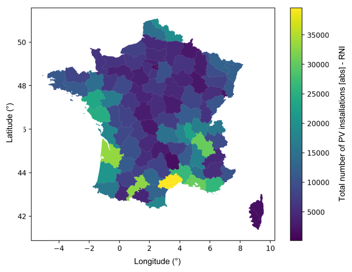
Figure 1
Map of the French department with the total number of PV installations below 36 kWp (source RNI).
PV Dataset (BDPV)
The “Asso BDPV” association, created in 2016, invites owners of RPV installations to provide information about the technical specifications of their installations so that their electricity production can be monitored using the data from the feed-in smart meter. The association also offers to verify their proper functioning by comparing production with other members’ installations or with a reference simulation. The association hosts and maintains the “BDPV “ (Photovoltaic Installation Database), which contains detailed characteristics and locations of more than 25,000 installations (BDPV, 2026).
Based on smart meter data, the daily RPV production of several thousand households was made available to this study by Asso BDPV.
Households’ description
The Household Heating Survey (HHS, originally Enquête Chauffage) was conducted by EDF in 2018. Its sample is representative of hexagonal France and was calibrated against the 2017 National Census (Insee, 2017), according to the following criteria: age and occupation of the household reference person; household size; dwelling type (single-family housing—detached, semi-detached or terraced—or multi-family buildings); occupancy status (owner or tenant); region ((Nomenclature of Territorial Units for Statistics NUTS 1); and agglomeration size.
The HHS provides a detailed, room-by-room description of each dwelling, enabling a high level of granularity regarding installed heating systems (e.g. nominal capacity, operational status) as well as time-varying indoor temperature setpoints.
Miscellaneous
Weather data derived from the ERA5 reanalysis dataset produced by the European Centre for Medium-Range Weather Forecasts (ECMWF), covering the period 1976–2018.
Models
Modelling PV production
The physics-based PV model was developed similarly to the choices made in (Kasmi, 2024) for a similar use case. Implementation was done using the PVLib library (F. Holmgren et al., 2018).
A photovoltaic system’s electrical output depends on incident solar irradiance, which includes direct (beam) and diffuse components. Meteorological datasets provide incident energy but not the solar position, which must be calculated based on the location. ERA5 data are for horizontal surfaces, but modules are tilted and oriented, so the plane-of-array (POA) irradiance calculation accounts for tilt and azimuth. Optical reflection losses are modelled using incidence angle modifiers that depend on the angle of incidence. Effective POA is the irradiance on the module surface. Thermal losses are modelled as a function of module temperature, which is influenced by irradiance, ambient temperature, and wind speed, thereby determining the direct current (DC) output.
In real installations, this DC power is subsequently processed by an inverter, which converts direct current into alternating current and adapts the voltage to ensure grid compatibility. These conversion processes entail additional losses, which the model represents through an inverter efficiency coefficient.
Modelling dwelling electricity consumption
The hourly power demand of each of the HHS households was computed using a combination of two bottom-up white-box dwelling stock energy models:
– For the thermal end-use load curve, the model is the one introduced in (Moreau et al., 2025). It has been validated against a representative empirical dataset of 6,000 load curves and exhibits a 3% normalised mean bias error (NMBSE) at the national scale.
– To compute the realistic behaviour of household and appliance electricity consumption, the SMACH agent-based model was used (Moussawel et al., 2025).
Methodology
Description of the rooftop PV stock
An initial data cleaning was performed on the BDPV to remove duplicate items, outliers, and other anomalies. The cleaned dataset was compared with the RNI and other available sources to identify potential biases in the representativeness of the whole stock.
Validation of the PV simulation
The main RPV characteristics (surface, peak power, tilt, and orientation) required for the simulation were extracted from the BDPV dataset.
The simulated daily RPV production was then compared with empirical production measured at the feed-in meter level for a sample of 1,000 RPV installations.
Self-consumption estimation
Once the production model is validated, various use cases have been simulated to assess the impact of rooftop photovoltaic (RPV) production on the 4,000-household sample representative of the French dwelling stock.
Some simplifying assumptions have been taken:
– Only SFH were considered in the use cases to avoid the complexity associated with collective self-consumption.
– The RPV characteristic used in each use case corresponds to the average values from the BDPV. The focus is thus on diversity arising from consumption rather than from a heterogeneous stock of RPV.
– For the sake of simplicity, an identical peak power value was assumed for every RPV in every use case (ranging from 1 kWp to 9 kWp depending on the use case).
– No DHW consumption is accounted for in the rest of this work. In France, electric domestic hot water (DHW) production can, in most cases, operate only during off-peak hours, which have changed significantly over the last few years. To avoid this complexity, only space heating and appliance consumption were modelled.
Results
The main characteristics of the residential RPV stock are first illustrated with the BDPV. These characteristics are then shown to be sufficient to model daily RPV production relative to empirical BDPV values accurately. A simulation at the whole residential scale is then carried out to match simulated consumption and production.
Description of the RPV stock
General overview
After cleaning, the BDPV contains information on 13,777 RPV installations. The average installation is 12 years old and has a peak power of 3.7 kWp. More than half of them are installed in the South of France.
Comparing the BDPV with the national register
While the results of this analysis are informative, they should be interpreted with caution, as they may be affected by selection bias due to the specific characteristics of the BDPV database. Membership in the BDPV association is entirely voluntary; consequently, potential biases may emerge regarding geographical location, system peak power or the socio-economic profile of owners.
As shown in Figure 2, most of the RPV installations in the BDPV were installed in the early 2010s. At the national scale, half of the stock was installed after 2022 according to France Territoire Solaire, meaning that the BDPV stock is much older than the average French stock (France Territoire Solaire, 2026). As a result, the average peak power in the BDPB (3.7 kWp) is below the average reported by the French DSO in late 2025 (4.5 kWp), as recent installations tend to be more powerful.
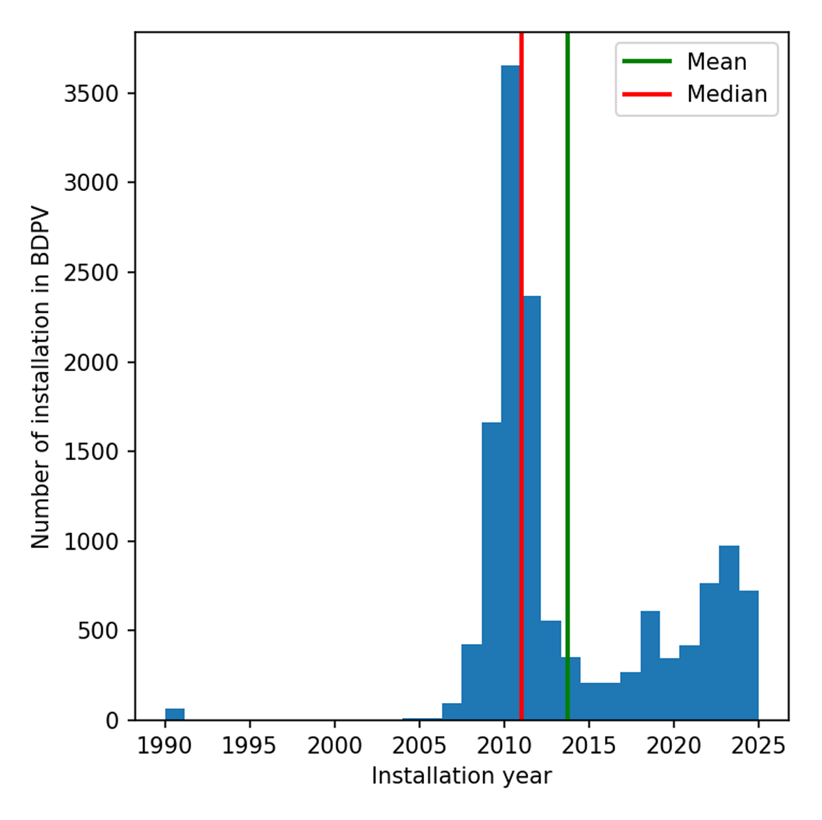
Figure 2
Distribution of the installation year of RPV installation in the BDPV.
For each department d, the proportion of installations recorded in the RNI that are also registered in the BDPV is calculated as follows and plotted in Figure 3:
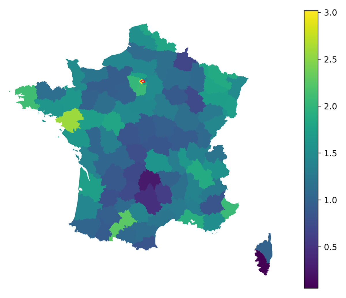
Figure 3
Ratio of installation in the BDPV dataset compared to the RNI.
Although the geographical distribution of residential installations recorded in the BDPV appears relatively uniform, a bias is nevertheless observed in the registration rate across departments. While explaining the origin of this bias lies beyond the scope of this study, it is essential to account for it in subsequent analyses. Consequently, the distribution of photovoltaic installations within the BDPV should not be considered fully representative of the national stock in France.
Descriptive statistics of the main variable of interest
Although this sample is not representative of the French RPV stock, it nevertheless provides useful insights into the main physical characteristics of RPV installation, namely:
Power: A very pronounced concentration is observed around 3 kWp in Figure 4. Indeed, among installations below 6 kWp, half have a peak capacity between 2.9 kWp and 3 kWp. This concentration is expected, as the analysis focuses on systems installed on individual houses, for which installations around 3 kWp were particularly common in France in the 2010s. The second peak around 6 kWp is typical of more recent installations.
Area: As for capacity, areas above 100 m² were aggregated for readability (60 systems). A strong concentration appears around 20 m² in Figure 5. For a 3 kWp system, this implies a specific power of 150 W/m², consistent with the typical performance of photovoltaic modules over the past decade.
Orientation: In Figure 6, 0° corresponds to north, 90° to east, 180° to south, and 270° to west. A very strong concentration at due south is observed, which, in the Northern Hemisphere, corresponds to the orientation that maximises annual yield. Peaks also appear at south-east, south-west, east and west orientations. These peaks are likely due to user approximation—either simplification or lack of precise knowledge of the system orientation—rather than exact correspondence.
Tilt: In Figure 7, 0° represents a horizontal installation and 90° a vertical one. Unlike the other parameters, no single value clearly dominates; instead, seven distinct tilt values emerge. The optimal tilt depends on latitude and on the period of the year during which production is prioritised. In France, a tilt of about 30° maximises annual production. However, the systems analysed here are mounted on residential rooftops. Although tilt adjustment using additional mounting structures is possible, it is rarely implemented due to simplicity and cost minimisation. These seven tilt categories most likely reflect the architectural diversity of the French building stock, as clearly visible in Figure 8. On the Atlantic coast and in mountainous areas, the slopes are steeper. Conversely, in southern France, roofs are traditionally flatter.
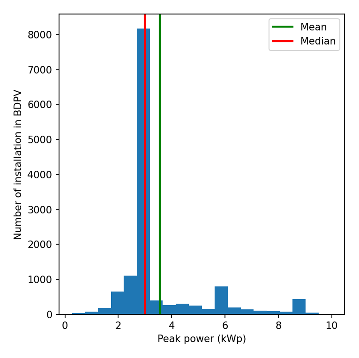
Figure 4
Distribution of peak power of RPV installations from the BDPV.
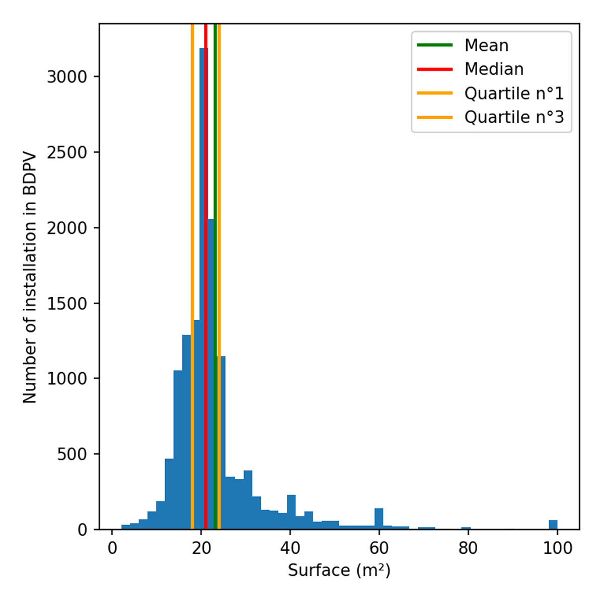
Figure 5
Distribution of the surface of RPV installations from BDPV.
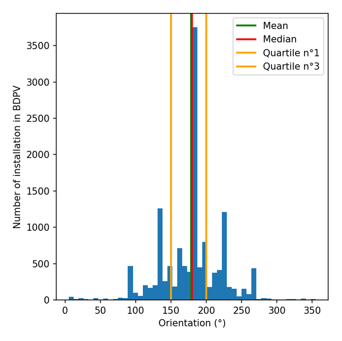
Figure 6
Distribution of orientation angle of RPV installations from BDPV (North = 0°, East = 90°, South = 180°, West = 270°).
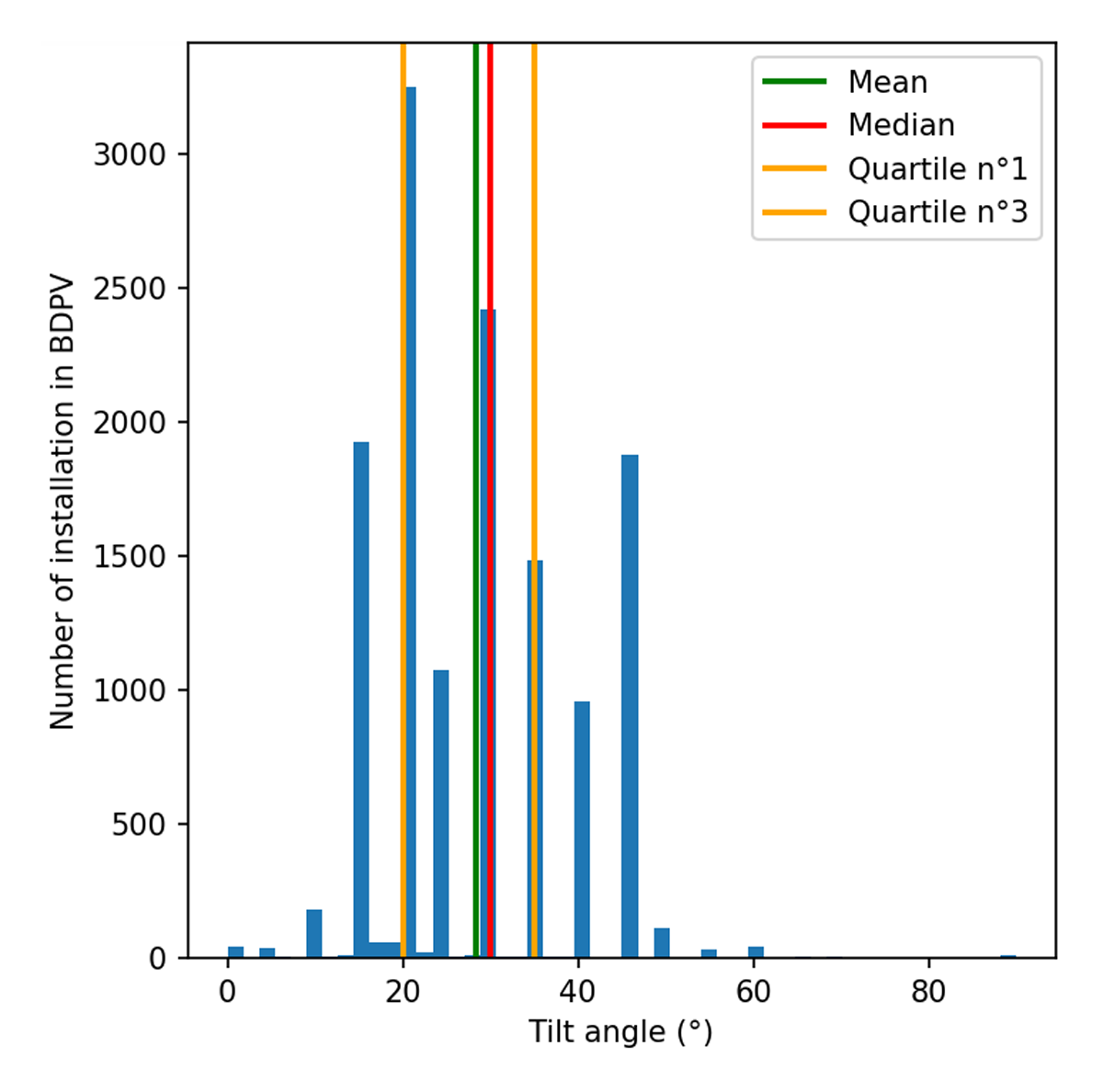
Figure 7
Distribution of tilt angle of RPV installations from BDPV.
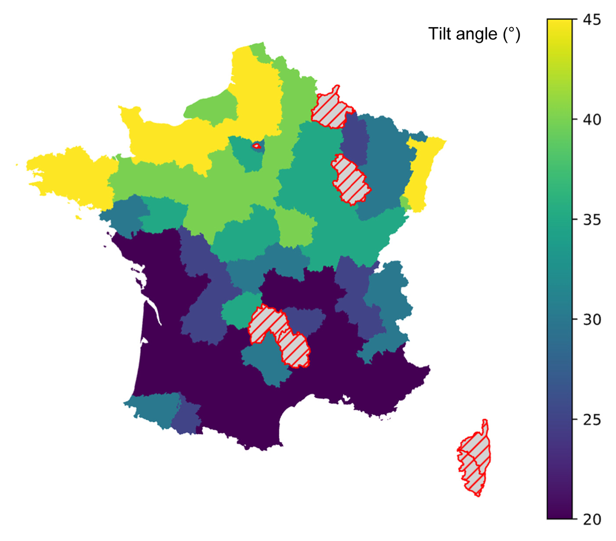
Figure 8
Map of the average tilt angle of RPV installation (°) per department from BDPV.
RPV model validation
Benchmark against an existing model
The RPV model developed in this study was first benchmarked against the PVGIS model (Gracia Amillo et al., 2021) for a 3 kWp panel, tilted at 30° and facing South. At an hourly time step, the model exhibits an NMBE (normalised mean bias error) of 5.5%, a CV(RMSE) (coefficient of variation of the root mean squared error) of 25%, and an R² of 0.98. These results are satisfactory given the calibration guidelines of the ASRHAE (American Society of Heating, Refrigerating and Air-Conditioning Engineers) as cited in (Ruiz and Bandera, 2017).
Empirical validation on BDPV
To enable comparison between the results and the observed production data, we contacted the BDPV association. A dataset was provided, comprising daily production data for several thousand installations over a three-year period. The anonymity of the households has been guaranteed, and the association members had previously consented to the disclosure of their production data for informational and research purposes. Confronting the simulation outputs with real-world measurements thus constitutes the final validation step of the modelling framework.
The adopted methodology consists of simulating the production of one thousand installations for which measured production data are available, using the technical parameters provided in the BDPV database. Subsequently, statistical performance indicators are computed, including the coefficient of determination (R²), the Normalised Mean Bias Error (NMBE), and the Coefficient of Variation of the Root Mean Square Error (CV(RMSE)), to quantify the agreement between simulated and observed production at the installation level.
Finally, average production curves derived from measurements and simulations are computed and compared. Given the substantial number of installations considered, this approach ensures robust representativeness across metropolitan France.
The superposition of the average measured and simulated daily production curves indicates that the simulation model performs satisfactorily at the daily time step (cf. Figure 9). However, this interpretation is only valid at the aggregated level. A linear regression line is therefore fitted to the data to provide a more robust assessment and to confirm the initial visual interpretation (Figure 10). To assess the model’s accuracy with greater rigour, it is necessary to compute similarity metrics for each installation to evaluate performance at the stock scale.
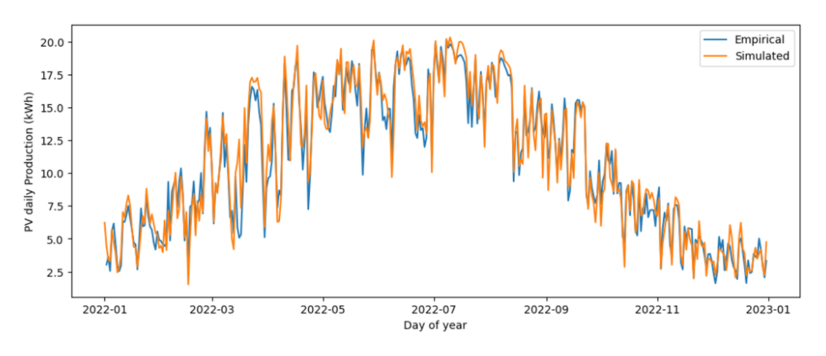
Figure 9
Average RPV daily production (kWh) for 1,000 installations from simulation (orange) and empirical measurement (blue) during the year 2022.
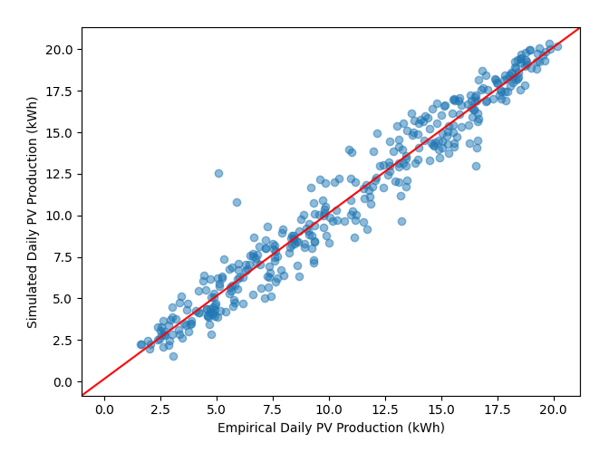
Figure 10
Average RPV daily production (kWh) for 1,000 installations from simulation as a function of empirical measurement value (kWh).
Table 1 shows the error for the average load curve compared to the average error for each individual load curve. The difference is typical of the error compensation that happened for the diversified production load curve. The distributions of error for each simulation vs. empirical production from the BDPV are plotted in Figure 11. The positive bias (16%) is typically due to PV panel ageing, masking effects, disruptions, etc., that are not accounted for in the model.
Table 1
Metrics between simulated and empirical RPV production. The first line is the metrics of the diversified load curve over 1,000 simulations. For the second line the metrics are computed across all individual simulations and then averaged.
| METRICS BETWEEN SIMULATED AND EMPIRICAL | R² | NMBE | CV(RMSE) |
|---|---|---|---|
| Metrics for the diversified production load curve | 0.95 | –0.01 | 0.11 |
| Average of the 1,000 individual metrics | 0.77 | 0.16 | 0.32 |
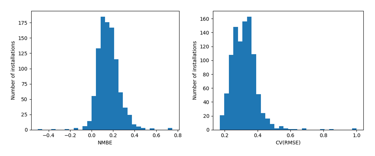
Figure 11
NMBE (left) and CV(RMSE) (right) distributions for the 1,000 simulated installations vs the empirical production from the BDPV. The left graph depicts the distribution of bias (NMBE) between simulation and empirical results of each of the 1,000 RPV installations.
Even though it can exhibit high error in individual installations, the choice of the model remains relevant for analysis at the aggregated level.
Production vs. consumption results at the stock scale
As introduced in the methodology section, for each representative SFH dwelling of the stock, the consumption load curve is then simulated at a 10-minute time step. The consumption is then matched with an RPV production. No behavioural changes to adapt consumption to the presence of PV are accounted for.
Metrics
The two following metrics are introduced, as proposed previously by many authors, as reviewed by (Luthander et al., 2015):
– Self-consumption, referring to the share of the PV production which is consumed on-site (PVc) normalised by the total PV production (PVtotal)
– Self-sufficiency, referring to the share of the consumption (P consumption, total) covered by the PV production consumed on-site (PVc):
Figure 12 illustrates these two metrics on a schematic PV production and consumption.
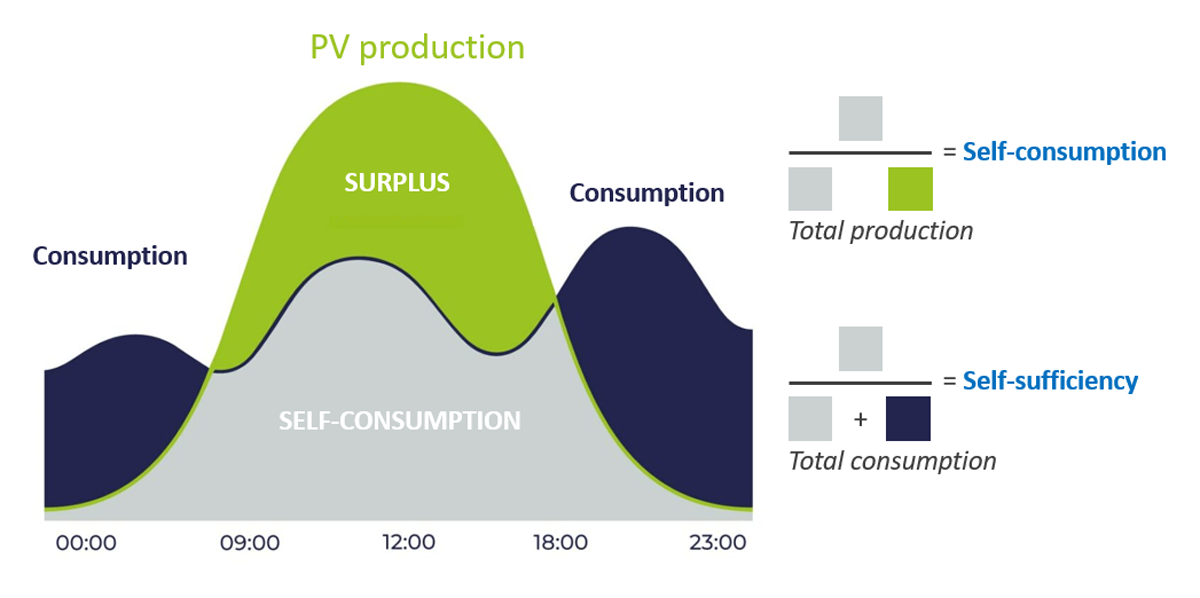
Figure 12
Schematic diagram of a PV production vs. consumption load curve and the associated metrics (self-consumption and self-sufficiency).
Results
Figure 13 shows the average load curves for an SFH dwelling with direct electric heating in winter (top) and in summer (bottom) for a few days. Space heating (red), appliances (blue) and total electric consumption (black) are compared with the RPV production (yellow). The dashed black line shows the difference between consumption and RPV production. In winter, space heating has a significant impact. Here, self-consumption reached 100%, while self-sufficiency is only 7%. On the contrary, during summer, self-sufficiency rises to 55% while self-consumption decreased to 56%, meaning a larger share of RPV production must either be curtailed or exported to the grid.
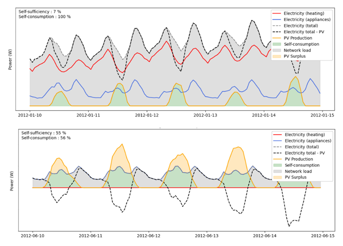
Figure 13
Simulated load curve for an average Joule-heated SFH of the stock. The Y-axis values have been removed for confidentiality reasons.
One may also note the variability in both consumption (due to behavioural differences from the agent-based model) and RPV production (due to weather), which is lower here because of the diversification brought by the average at the stock scale.
This diversity is further illustrated in Figure 14, which shows the distribution of self-sufficiency and self-consumption for each day and each SFH dwelling of the stock. The following observation can be made:
– The spread of self-consumption is much higher than the self-sufficiency. The interquartile range (IQR) is twice as wide (self-consumption IQR of 14% vs. self-sufficiency IQR of 7%).
– During summer, self-sufficiency increases due to higher RPV production and lower consumption (especially for electrically heated dwellings), while self-consumption share decreases due to RPV surplus.
– A slight negative correlation exists between self-sufficiency and self-consumption, as dwellings with higher overall consumption tend to show both higher self-consumption and lower self-sufficiency. For example, as summarised in Table 2, in January, households with electric heating have an average of 89% self-consumption and 10% self-sufficiency, compared to 70% self-consumption and 20% self-sufficiency for non-electric space heating.
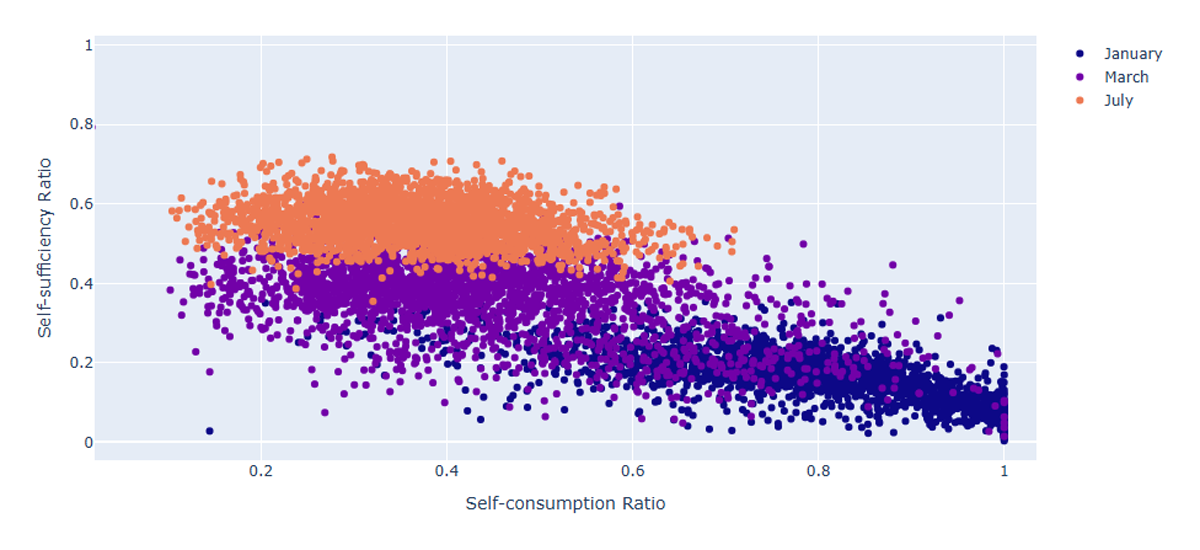
Figure 14
Self-sufficiency as a function of self-consumption. The metrics are computed for every day and every dwelling of the stock for the month of January (orange), March (purple) and July (orange).
Table 2
Average values of self-sufficiency and self-consumption per type of space heating (electric/non-electric) with a 3 kWp RPV installation.
| METRIC | MONTH | NON-ELECTRIC SPACE HEATING | ELECTRIC SPACE HEATING |
|---|---|---|---|
| Self-sufficiency | January | 20% | 10% |
| July | 55% | 55% | |
| Self-consumption | January | 73% | 89% |
| July | 37% | 36% |
The sensibility to installed peak power was then examined, varying from 1 to 9 kWp. The results are summarized in Table 3. In winter, increasing the installed peak power increase the self-sufficiency as PV production remains below consumption. In summer, a non-linearity is identified: part of the consumption remains at night, so self-sufficiency thus remains below 64%. On the contrary, self-consumption decreases in summer when peak power increases (72% to 15%) because it yields PV surplus.
Table 3
Average self-sufficiency and self-consumption by month for SFH with non-electric space heating as a function of the RPV peak power.
| METRIC | MONTH | RPV PEAK POWER PER DWELLING | |||
|---|---|---|---|---|---|
| 1 KWp | 3 KWp | 6 KWp | 9 KWp | ||
| Self-sufficiency | January | 10% | 20% | 26% | 29% |
| February | 21% | 32% | 37% | 39% | |
| March | 29% | 42% | 46% | 48% | |
| April | 31% | 47% | 53% | 56% | |
| May | 36% | 53% | 59% | 62% | |
| June | 36% | 54% | 61% | 64% | |
| July | 38% | 55% | 62% | 64% | |
| Self-consumption | January | 93% | 73% | 56% | 45% |
| February | 80% | 50% | 33% | 24% | |
| March | 72% | 39% | 23% | 16% | |
| April | 75% | 42% | 25% | 18% | |
| May | 72% | 39% | 23% | 16% | |
| June | 75% | 41% | 25% | 18% | |
| July | 72% | 37% | 21% | 15% | |
Discussion
Stock description
Dealing with multiple data sources (RNI, BDPV …) is inherently challenging due to inconsistencies arising from differences in scale (representative vs voluntary sample), the type of data provided (aggregated vs detailed), etc. While BDPV exhibits good geographical representativity, its inherent bias should be kept in mind.
– Households currently equipped with RPV are not representative of the overall population. They tend to have higher incomes, own their homes, are often retired, and exhibit higher-than-average electricity consumption, as identified in Denmark (Hansen et al., 2022).
– Additionally, BDPV installations are older, so the distribution of peak power of BDPV’s installation reflects historical old feed-in tariffs, leading to more installations below 3 kWp. According to (France Territoire Solaire, 2026), almost half of recent installations are between 3 kWp and 9 kWp.
– Future RPV stock may be different from the current one. For example, most existing installations are south facing, but the share of available roofs optimally oriented to the south may be lower in the future.
PV modelling
The simplified modelling implemented in this study, based on Dobos, is satisfactory at the aggregated scale (Dobos, 2014). However, due to limited information on shading, exact installation characteristics and other factors, significant dispersion occurs at the individual scale. A higher error would be expected at an hourly time step if high-resolution empirical data were available.
Some biases can be attributed to the use of ERA5 weather solar irradiance, which is known to exhibit high biases relative to satellite imagery (Wilczak et al., 2024). Effects such as panel ageing or disruption were not included and may explain the compensation error at the aggregate scale.
Validation in this study was limited to PV production. Future validation should also consider the net load, using sufficient empirical load curves from households with and without PV.
Impact of PV adoption on load curves
In this work, the net load was computed by subtracting PV production from the consumption load curve. No specific household behaviour having RPV was assumed, such as shifting consumption when PV is available or the “solar rebound” effect (Bigler, 2025).
Moreover, the effect of devices that could maximise self-sufficiency, such as Home Energy Management Systems (HEMS) or storage systems like stationary batteries and EVs, should be considered as proposed by (Van Der Kam et al., 2024).
Conclusion
This work proposes a description of the existing stock of RPV panels in SFH in France, with sufficient detail to enable their simulation in a BSEM. This description relies largely on the BDPV dataset and thus inherits its associated biases.
Based on empirical PV production data from BDPV, a physics-based PV panel simulation model was then validated at an aggregated level.
The simulated PV production was then paired with consumption load curves derived from the building stock energy model. Self-sufficiency and self-consumption metrics were then computed for various RPV characteristics, accounting for the diversity of SFH dwellings.
Future work
Future work will include modelling household behaviour in the agent-based model when PV production is available, to assess the amount of energy displaced by households with RPV.
The upcoming update to the CONSER survey (Binet and Cayla, 2019) is also expected to include questions on RPV installations, such as “plug and play” devices and storage systems. This will enable a better linkage between household characteristics and their RPV installation.
Additionally, a survey on self-consumption practices is planned to improve understanding of behaviours and constraints related to RPV installations.
The net load of a household with an RPV could then be validated against an empirical net load curve, allowing for a more realistic assessment of the long-term impact of PV self-consumption in a national BSEM.
Additional File
The additional file for this article can be found as follows:
PowerPoint Slides
PowerPoint Slides relating to this article. URI: https://eceeeproceedings.org/articles/50/files/6a58af4b2b573.pdf
Notes
Data Accessibility Statement
The authors do not have permission to share data.
Author Contributions
The authors performed the following contributions:
– Valentin Moreau: Visualization, Writing – original draft, Methodology, Supervision
– Evan Grimaud: Formal analysis, Visualization, Writing – original draft
– Guillaume Binet: Conceptualization, Supervision, Writing – review & editing
– Yves-Marie Saint-Drénan: Data curation, Writing – review & editing
– David Trebosc: Data curation
– Durca Pathmanathan: Project administration, Writing – review & editing
eceee paper ID
4-187-26