
Table 1
Summary of dataset variables.
| VARIABLE | UNIT | RANGE | MEAN | |
|---|---|---|---|---|
| Type of dwelling | category | MFHSFH | 16%84% | |
| Floor area | m² | 50–250 | 115 | |
| Household size | unit | 1–6 | 2.37 | |
| Type of AAHP installed | category | monosplitmultisplit | 32.9%65.9% | |
| Space heating in the post-situation | Post-REH use | % | 0–100 | 9.75 |
| Post-AAHP use | % | 50–100 | 86.2 | |
| Post-wood stove | % | 0–50 | 2.6 | |
| Post-fireplace | % | 0–50 | 1.8 | |
| Post-other | % | 0–30 | 0.6 | |
| Space heating in the pre-situation | Pre-REH | % | 0–100 | 83.9 |
| Pre-boiler | % | 0–100 | 3.4 | |
| Pre-biomass | % | 0–50 | 5.4 | |
| Pre-other | % | 0–100 | 7.2 | |
| Air-conditioning in the post-situation | category | yes | 86.3% | |
| Additional retrofit | category | yes | 22.7% | |
| Domestic hot water | Electric water heater | category | yes | 79.5% |
| Thermodynamic water heater | category | yes | 18.2% | |
| Solar water heater | category | yes | 1.1% | |
| Boiler | category | yes | 1.1% | |
| Photovoltaic panel | category | yes | 5.7% | |
| Average daily consumption for outdoor temperature in the range [–1°C, 1°C] | kWh/day | 0.02–150 | 59 | |
| Heating Degree Days | °C.days | 1,318–3,982 | 1,938 | |
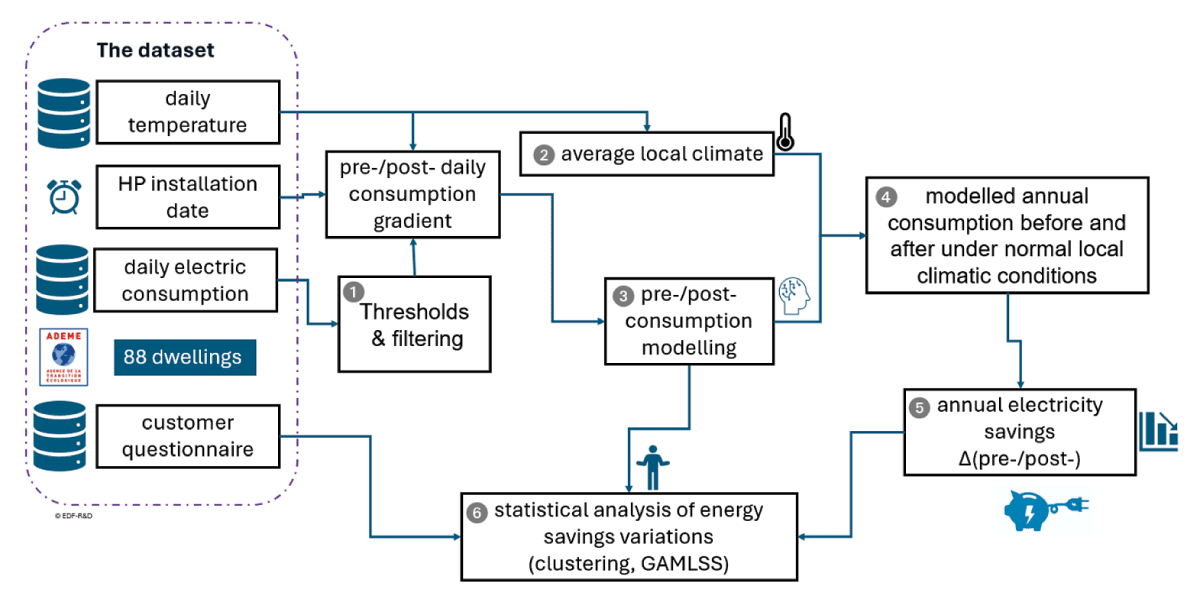
Figure 1
Synthesis of the methods used.
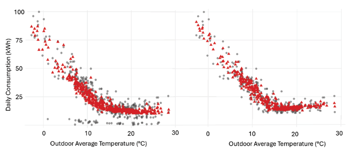
Figure 2
Example of data cleaning removing low consumption and impact on modelled values. Left: before, right: after. In red: modelled, in grey: metered values.
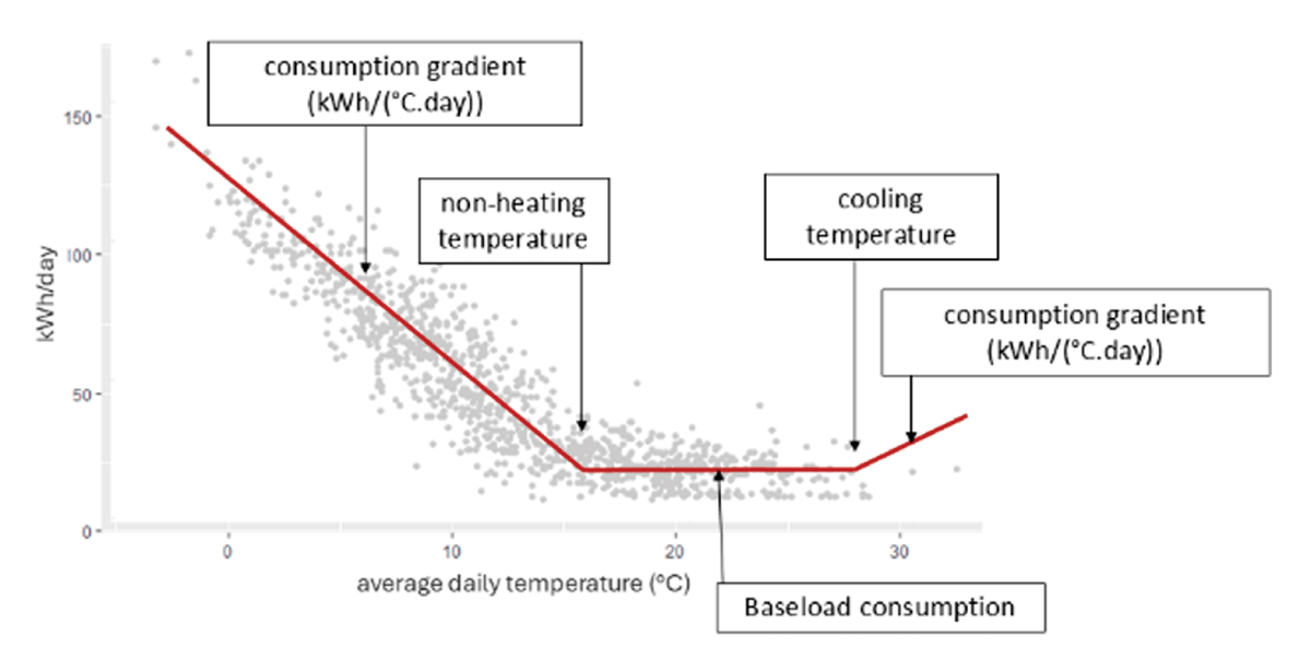
Figure 3
Schematic representation of the daily consumption gradients (all end-uses), non-heating temperature threshold and cooling temperature (tipping points) (Osso et al. 2024).
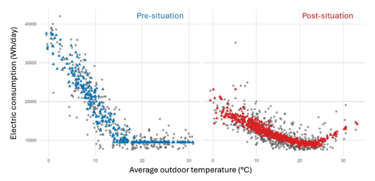
Figure 4
Example of daily consumption modelling pre- and post-situation of AAHP installation. Left blue: pre-modelled, right red: post-modelled, in grey: metered values.
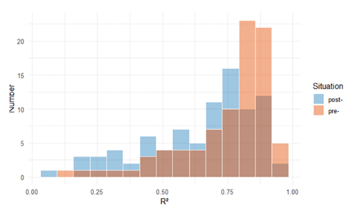
Figure 5
Histogram of the coefficient of determination (R²) of the EARTH models in pre- and post-situation. R² mean: pre- = 0.749, post- = 0.652.
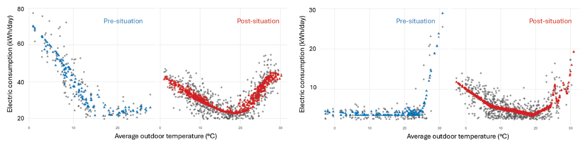
Figure 6
Examples of new uses (left) for air conditioning in the post-situation (red) and pre-existing air conditioning (right) in the pre-situation (blue).
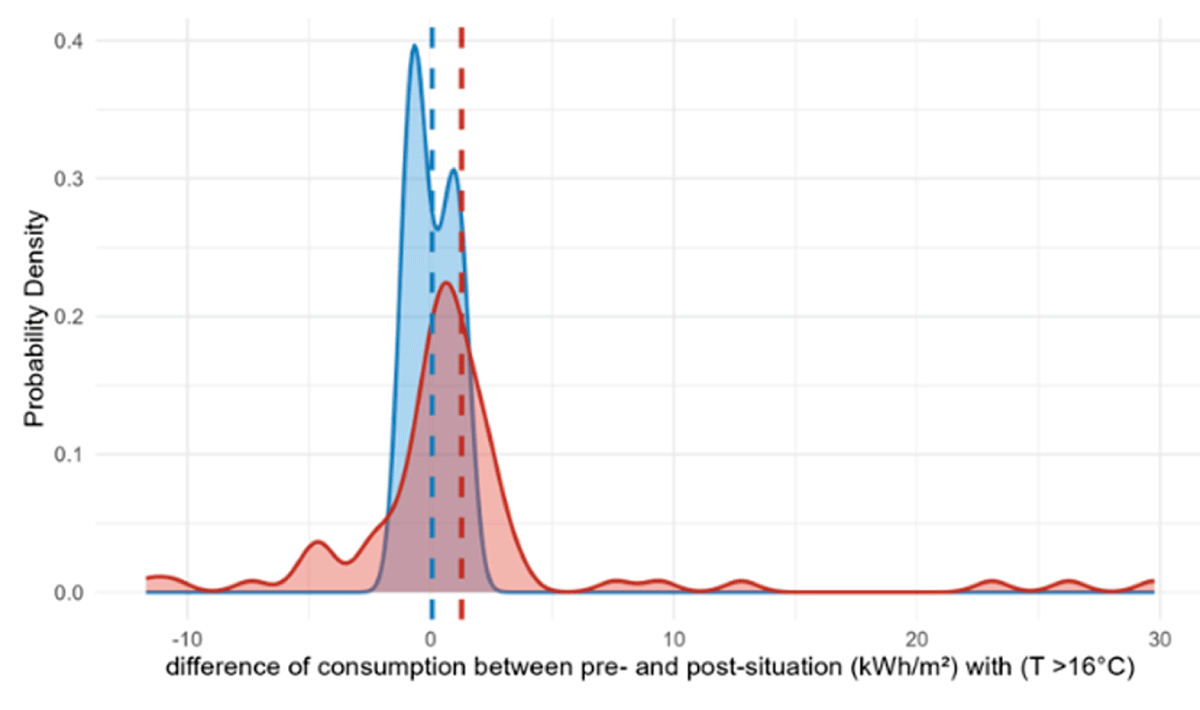
Figure 7
Distribution showing the increase in consumption (in kWh/m²) between the pre- and post-situations, with an average daily outdoor temperature above 16°C, based on the respondent’s reported use of air-conditioning (AC-yes in red, AC-no in blue). Dashed lines = mean value.
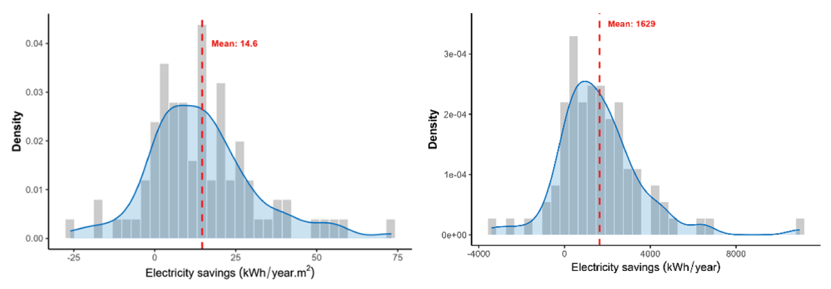
Figure 8
Histogram of the assessed electricity savings (left: ESU in kWh/(m².year)), (right: ES in kWh/year). All end-uses electricity savings including air-conditioning and gas boiler to AAHP switch (i.e. negative savings).
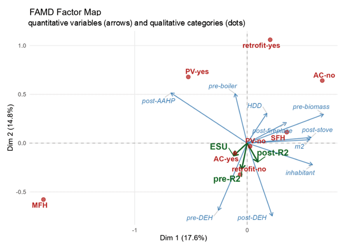
Figure 9
Visualisation of the correlation coefficients between variables and the principal components (the first two axes). In blue: quantitative variable, in red: qualitative variables, in green: additional variables. The quantitative variables are represented as arrows on these axes: the longer the arrow and the closer it is to an axis, the more closely the variable is linked to that axis. Categorical variables are represented by dots: two categories that are close to each other in the space indicate similar profiles in the data. ESU, R² are included as illustrative variables.
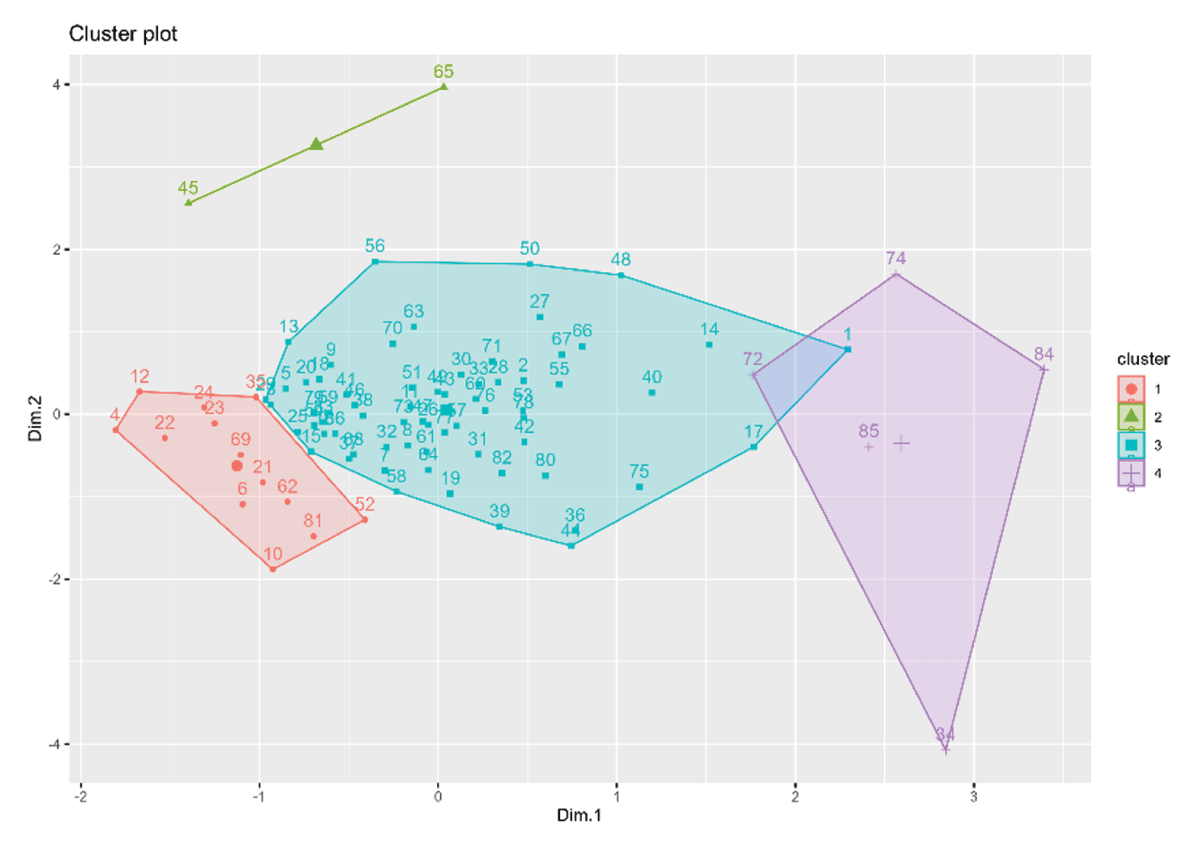
Figure 10
Cluster visualization (HCPC) in the FAMD map (the first two axes). Projection of individuals onto the first two dimensions of the FAMD. Observations are grouped into four clusters identified via Hierarchical Clustering on Principal Components (HCPC). Proximity: Points located close to each other represent individuals with similar characteristics or survey responses. The two main axes (Dim 1 & Dim 2) summarize most of the variation in the dataset (see Figure 9).
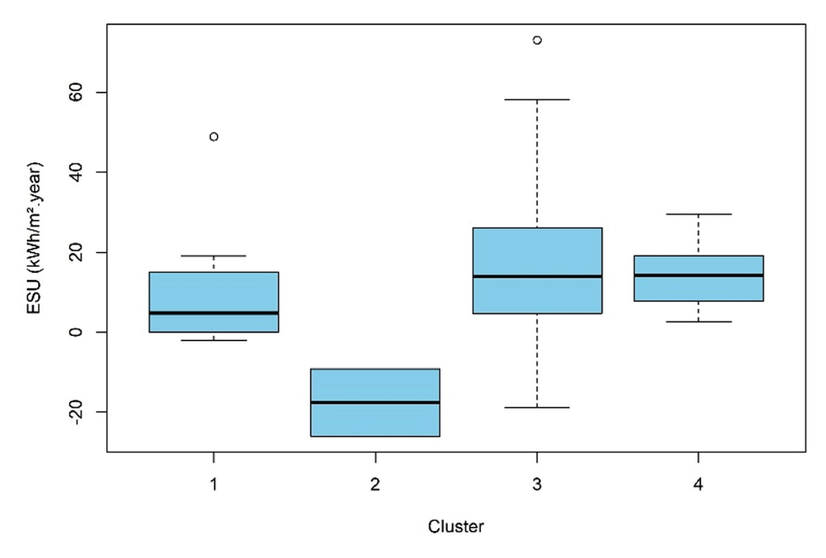
Figure 11
Boxplot of electricity savings (ESU in kWh/(m².year)) per HCPC cluster.
Table 2
GAMLSS model of the annual electricity savings (ES in kWh/year). Explanatory variables are normalised.
| ESTIMATE | STD. ERROR | t-VALUE | p-VALUE | |||
|---|---|---|---|---|---|---|
| µ coefficients(mean) | (Intercept) | 1699.0 | 306.0 | 5.553 | 4.18e–07 | *** |
| Household size (unit) | –328.5 | 112.5 | –2.918 | 0.00466 | *** | |
| Daily consumption during cold days (T = [–1°C, 1°C]) (kWh/day) – pre-situation | 975.7 | 196.7 | 4.959 | 4.37e–06 | *** | |
| σ coefficients(variance) | (Intercept) | 6.9206 | 0.1491 | 46.428 | <2e–16 | *** |
| Daily consumption during cold days (T = [–1 °C, 1 °C]) (kWh/day) – pre-situation | 0.3451 | 0.1307 | 2.641 | 0.0101 | * | |
| Floor area (m²) | 0.2629 | 0.1364 | 1.928 | 0.0576 | . | |
| υ (skewness) | (Intercept) | –0.008775 | 0.15704 | –0.056 | 0.956 | |
| τ (kurtosis) | (Intercept) | 1.5300 | 0.57773 | 2.65 | 0.00983 | ** |
[i] Only significant variables are presented, others as presented in Table 1, are not significant or collinear with the selected variables (see Table 13 in Annex).
Note: *p < 0.05, **p < 0.01, ***p < 0.001.
No. of observations in the fit: 83 – Degrees of Freedom for the fit: 9.
Residual Deg. of Freedom: 74 – Global Deviance: 1,421.897 – AIC: 1,439.897 – SBC: 1,461.666.
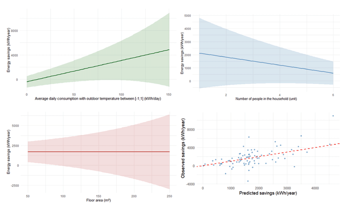
Figure 12
Marginal effect of explanatory variables on the predicted mean (µ), with a 95% prediction interval incorporating the dispersion parameter (σ). Bottom right: observed values versus predicted values, red dashed line: perfect fit.
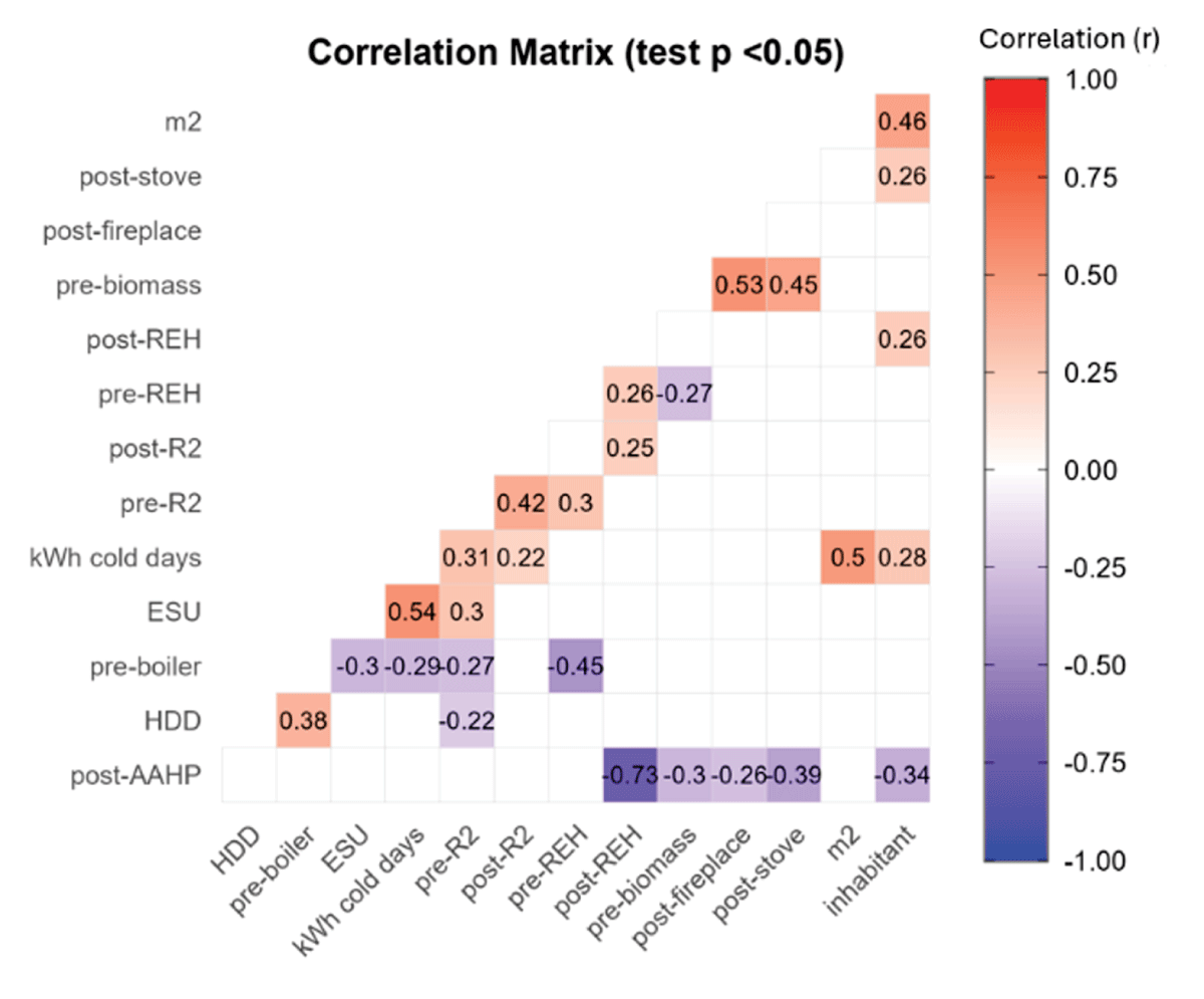
Figure 13
Correlation matrix between the variables studied. Only statistically significant correlations at the threshold are displayed. The empty spaces correspond to non-significant coefficients (p ≥ 0.05).
Table 3
Principal component analysis – Eigenvalues (variance explained).
| VARIANCE | % OF VAR. | CUMULATIVE % OF VAR. | |
|---|---|---|---|
| Dim. 1 | 2.470 | 17.641 | 17.641 |
| Dim. 2 | 2.067 | 14.766 | 32.407 |
| Dim. 3 | 1.579 | 11.276 | 43.683 |
| Dim. 4 | 1.452 | 10.375 | 54.057 |
| Dim. 5 | 1.285 | 9.176 | 63.233 |
Table 4
Characterization of clusters resulting from hierarchical ascending classification on principal components (HCPC).
| DISCRIMINANT QUANTITATIVE VARIABLES (v-TEST) | ||||||
|---|---|---|---|---|---|---|
| VARIABLE | v.TEST | MEAN IN CATEGORY | OVERALL MEAN | SD IN CATEGORY | OVERALL SD | p.VALUE |
| Cluster#1 | ||||||
| pre-REH | 2.006 | 100 | 85.05 | 0.00 | 28.967 | 4.476451e–02 |
| m² | 3.921 | 75 | 115.67 | 18.518 | 40.358 | 8.813829e–05 |
| Cluster#2 | ||||||
| Pre-boiler | 9.218 | 100.00 | 2.348 | 0.00 | 15.069 | 3.009722e–20 |
| HDD | 3.513 | 2908.4 | 1937.91 | 1074.4 | 392.90 | 4.414451e–04 |
| pre-R² | –2.486 | 0.464 | 0.756 | 0.341 | 0.167 | 1.291103e–02 |
| ESU | –2.719 | –17.611 | 14.647 | 8.443 | 16.872 | 6.528922e–03 |
| pre-REH | 4.177 | 0.00 | 85.05 | 0.00 | 28.967 | 2.950168e–05 |
| Cluster#3 | ||||||
| m² | 3.568 | 124.272 | 115.67 | 39.936 | 40.358 | 0.0003594492 |
| post-AAHP | 2.393 | 87.454 | 85.139 | 10.812 | 16.197 | 0.0166776343 |
| post-stove | –2.295 | 1.363 | 2.616 | 4.650 | 9.141 | 0.0217311903 |
| pre-boiler | 2.576 | 0.030 | 2.348 | 0.244 | 15.069 | 0.0099715353 |
| Cluster#4 | ||||||
| post-stove | 6.110 | 27.0 | 2.616 | 22.715 | 9.141 | 9.957710e–10 |
| pre-biomass | 4.804 | 30.6 | 5.209 | 18.039 | 12.104 | 1.548102e–06 |
| post-fireplace | 2.952 | 10.0 | 1.662 | 20.00 | 6.467 | 3.148761e–03 |
| inhabitant | 2.223 | 3.4 | 2.371 | 1.743 | 1.059 | 2.619405e–02 |
| post-AAHP | 6.100 | 42.0 | 85.139 | 21.354 | 16.197 | 1.055582e–09 |
[i] The mean in category indicates the average value within the cluster, compared to the overall mean of the sample. The clusters were characterized using the v-test. A variable is considered characteristic of a cluster if the difference between its intraclass mean and its overall mean is statistically significant, which corresponds to a |v-test| ≥ 1.96 (equivalent to a threshold of p < 0.05).
Table 5
Characterization of clusters by qualitative variables (HCPC).
| DISCRIMINATING QUALITATIVE CRITERIA (v-TEST) | |||||
|---|---|---|---|---|---|
| CATEGORY | CLA/MOD | MOD/CLA | GLOBAL | p.VALUE | v.TEST |
| Cluster#1 | |||||
| MFH | 92.857 | 100 | 16.279 | 1.608517e–14 | 7.678588 |
| SFH | 0.000 | 0 | 83.720 | 1.608517e–14 | –7.678588 |
| Cluster#2 | |||||
| Non significant | |||||
| Cluster#3 | |||||
| SFH | 91.666 | 100 | 83.720 | 8.540566e–12 | 6.829173 |
| MFH | 0.000 | 0 | 16.279 | 8.540566e–12 | –6.829173 |
| Cluster#4 | |||||
| Nonsignificant | |||||
[i] Cla/Mod (Percentage of the Cluster in the Category): Proportion of individuals with this category in the cluster (measure of specificity). Mod/Cla (Percentage of the Category in the Cluster): Proportion of individuals in the cluster with this category (measure of representativeness). Global: Relative frequency of the category in the entire sample. v-test Standardized score, a|v-test| ≥ 1.96 indicates a statistically significant representation of the category within the cluster compared to the overall average.
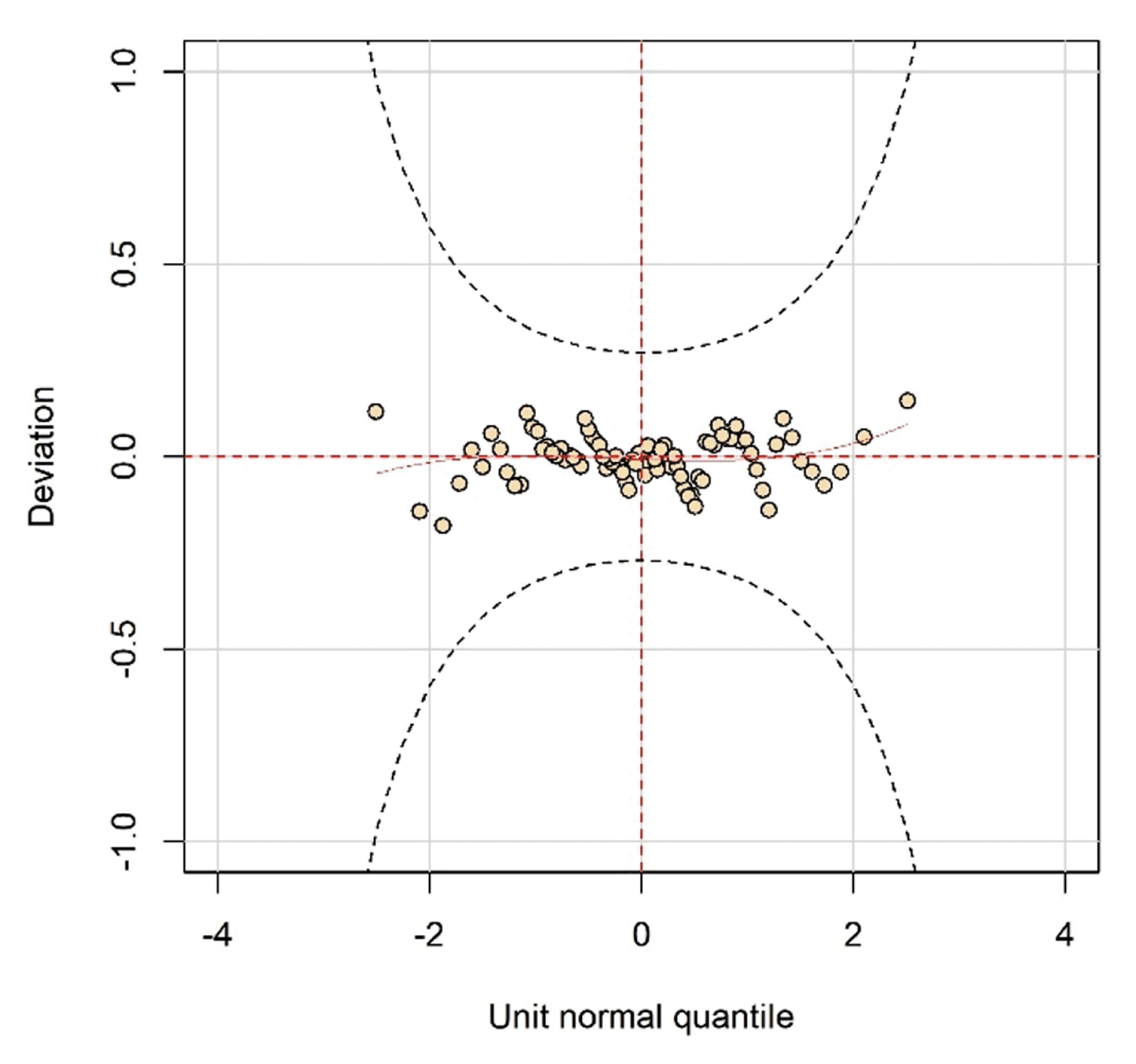
Figure 14
Worm plot (van Buuren & Fredriks 2001) of the normalised quantile residuals for the GAMLSS model. The Deviation axis represents the difference between the observed and theoretical quantiles. The horizontal elliptical curves represent the 95% confidence limits. The flat shape of the red trend line and the inclusion of all residuals within the confidence bands indicate an adequate model fit, capturing the location, scale, and shape parameters of the response variable distribution.