
Introduction
Electrification and energy demand reduction are two central pillars of the global energy transition, complemented by the imperative to adapt to climate change. As highlighted by the Intergovernmental Panel on Climate Change (IPCC 2022), electrification is expected to be the primary strategy for decarbonizing building energy end-uses such as heating and cooking. Under the REPowerEU plan, heat pumps play a crucial role in reducing carbon emissions and decreasing reliance on imported fossil fuels (Toleikyte et al. 2023).
In France, according to the trade association UNICLIMA, approximately 800,000 air-to-air heat pumps (AAHPs) – 34% of which were multi-split systems – and 179,000 air-to-water heat pumps (AWHPs) were sold in 2025 (UNICLIMA 2026). Both technologies belong to the air-source heat pump (ASHP) family. Despite these sales, electric space heating in French residential buildings remains dominated by resistive electric heating (REH). REH accounts for 37.2% of the residential building stock, whereas heat pumps of all types represent only 5.1%. In 2023, residential electric space heating represented approximately 43.5 TWh, compared with a total space-heating demand of 253.7 TWh across all energy carriers in metropolitan France (SDES 2026).
Replacing REH with AAHPs offers substantial energy efficiency potential. Although the associated greenhouse gas (GHG) reductions are lower than those achieved by replacing fossil fuels – given the low carbon intensity of the French electricity grid1 (51.9 gCO2eq/kWh; ADEME 2024) – the total energy savings remain significant.
Comprehensive reviews of ASHP field trials are available in Miara, Günther, and Langner (2021) and Carroll, Chesser, and Lyons (2020), while Jiang, Zhao, and Ni (2025) provide a bibliometric analysis of research in this domain from 1985 to 2022.
However, most European field studies focus on AWHPs (e.g., ADEME et al. 2025 in France). To our knowledge, few studies examine the replacement of REH by AAHPs in European residential buildings. This gap is understandable because REH is not the dominant space-heating technology across Europe, where natural gas boilers prevail. REH represents 31% of the residential stock in Spain, 18% in the UK, and 17.5% in Italy, while heat pump penetration remains low (1% in the UK, 15% in Italy and Spain; MSI Group 2025). The main exceptions are Nordic countries (Sweden, Finland, and Norway), where heat pumps account for over 40% of space heating systems (Rosenow et al. 2022).
Historically in France, AAHPs have been viewed primarily as air-conditioning units rather than space heating systems, with monthly sales spiking after heatwaves (Uniclima 2026). Air conditioning is sometimes criticized as an inefficient adaptation strategy due to its energy intensity (ESABCC 2026). In a European survey, over 38% of respondents reported an inability to keep their homes adequately cool during summer (EEA 2026). Nevertheless, because AAHPs are reversible (providing both heating and cooling), their high efficiency during winter can largely outweigh the additional electricity consumed for summer cooling.
In France, air-conditioning penetration rates are estimated to range between 18% and 26% of dwellings. Yet, cooling represents only ~1% of total residential electricity demand due to sporadic operational patterns (ADEME 2025). Portable air conditioners accounted for 40% of the cooling stock in 2020 and are energy intensive (CODA 2021).
Binet and Grignon-Massé (2020) observed that portable units were used for 77 days per year, consuming over 850 kWh/year, compared to 110 days and 460 kWh/year for reversible AAHPs. On the contrary, the ADEME and ENETECH (2025) study gives much lower values, with much smaller differences in consumption between fixed and portable units (respectively 136 kWh/year and 160 kWh/year). The study highlights the need to conduct measurement campaigns on larger sample sizes to draw more robust conclusions, due to the small size of the current panel.
In this context, we conduct an ex-post assessment of the electricity savings (ES in kWh/year) resulting from the retrofitting of REH (the “Joule”2 baseline) with an AAHP (the “Carnot” retrofit3). This study extends an initial report by Dupret (2025) by applying advanced statistical techniques to the same empirical dataset. In a previous pilot study (Osso et al. 2024), we evaluated statistical methods on a single case study. Here, we extend that analytical framework to a sample of 88 households undergoing the same type of retrofit.
Due to data constraints, this study does not allow the estimation of the performance of heat pumps (COP), nor the impact of individual building characteristics on overall savings. This study provides quantitative evidence regarding actual electricity savings observed in the field, rather than estimates based on the measured or theoretical performance of AAHPs.
Marchal (2026) and Staffell et al. (2012) explain that a heat pump’s intrinsic COP must be distinguished from a dwelling’s actual heating energy consumption. Actual performance depends on equipment settings, installation quality, water flow temperature, sizing, and heat emitters, rather than the building’s thermal envelope. Therefore, a high COP does not automatically translate into low energy consumption. This study aims to address this point, moving beyond mere nominal performance to examine actual savings.
The remainder of this paper is structured as follows: Section 2 describes the dataset. Section 3 details the analytical methodology. Section 4 presents the empirical results, including normalised electricity savings per unit of floor area (ESU, in kWh/(m².year)), cluster analysis, and distributional savings modelling. Section 5 discusses policy and technical implications.
Surveyed households
The dataset originates from a field study on AAHPs conducted by ADEME (Dupret 2025), in which installations were subsidized through the French Energy Efficiency Obligation (EEO) scheme (MTE 2026; Gonand 2024). A detailed description of the 88 households surveyed is presented in Dupret (2025), and only a summary is provided here. The dataset is non-representative of the French residential building stock and does not incorporate weighting factors to ensure representativeness.
According to the survey responses, 84% of households live in single-family housing (SFH) and the remaining 16% in multifamily housing (MFH). The average floor space is 115 m² (MFH = 74 m², SFH = 123 m²) and the average household size is 2.37 people (MFH = 1.96, SFH = 2.45).
Table 1
Summary of dataset variables.
| VARIABLE | UNIT | RANGE | MEAN | |
|---|---|---|---|---|
| Type of dwelling | category | MFHSFH | 16%84% | |
| Floor area | m² | 50–250 | 115 | |
| Household size | unit | 1–6 | 2.37 | |
| Type of AAHP installed | category | monosplitmultisplit | 32.9%65.9% | |
| Space heating in the post-situation | Post-REH use | % | 0–100 | 9.75 |
| Post-AAHP use | % | 50–100 | 86.2 | |
| Post-wood stove | % | 0–50 | 2.6 | |
| Post-fireplace | % | 0–50 | 1.8 | |
| Post-other | % | 0–30 | 0.6 | |
| Space heating in the pre-situation | Pre-REH | % | 0–100 | 83.9 |
| Pre-boiler | % | 0–100 | 3.4 | |
| Pre-biomass | % | 0–50 | 5.4 | |
| Pre-other | % | 0–100 | 7.2 | |
| Air-conditioning in the post-situation | category | yes | 86.3% | |
| Additional retrofit | category | yes | 22.7% | |
| Domestic hot water | Electric water heater | category | yes | 79.5% |
| Thermodynamic water heater | category | yes | 18.2% | |
| Solar water heater | category | yes | 1.1% | |
| Boiler | category | yes | 1.1% | |
| Photovoltaic panel | category | yes | 5.7% | |
| Average daily consumption for outdoor temperature in the range [–1°C, 1°C] | kWh/day | 0.02–150 | 59 | |
| Heating Degree Days | °C.days | 1,318–3,982 | 1,938 | |
Prior to retrofitting, space heating was supplied primarily by REH alone (67%) or REH combined with biomass (wood stoves or fireplaces, 28.4%). Three households used a gas boiler, and one used REH alongside a gas boiler. Following the retrofit, all installed AAHPs were split systems (mono- or multi-split). Although only 28.4% of households rely exclusively on the AAHP for heating, AAHPs cover 87% of the total heated floor space on average, while residual REH covers 9% and biomass covers 4% (Dupret 2025).
Furthermore, 86.3% of respondents reported using their new AAHP for summer cooling. Prior air-conditioning usage data were unavailable.
Finally, 22.7% of households performed additional envelope retrofits during the monitoring period, and 5.7% had photovoltaic panels installed (compared to the national average of 1.6%; Ecoinfo 2022). Self-consumption rates for PV generation were not recorded.
Methods
The analytical framework consists of six stages implemented in the R statistical environment (R Core Team 2025), as summarized in Figure 1:
Data processing, including data cleaning (step 1) and local normal climate calculation (step 2).
Daily consumption (DC) modelling using multivariate adaptive regression splines (step 3).
Assessment of electricity savings (ES) at normal local climate using DC modelling (step 4 and 5).
Statistical analysis of electricity savings per floor area unit (ESU) variations by clustering and ES modelling based on questionnaire variables (step 6).
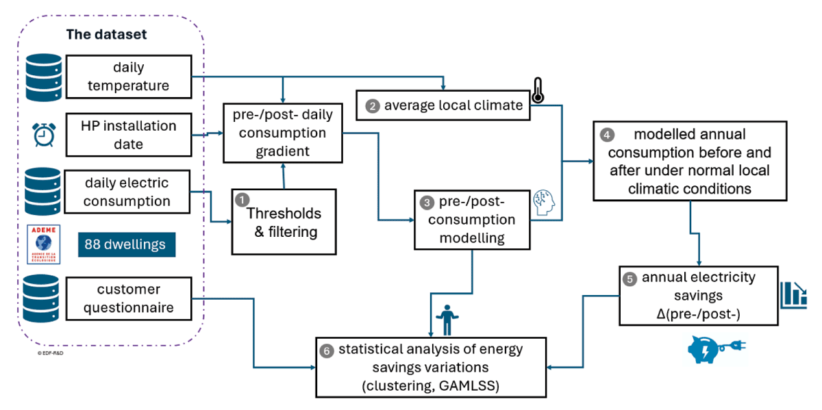
Figure 1
Synthesis of the methods used.
In summary, for each dwelling, we model local climate and daily electricity consumption with AAHP heating and REH heating, to estimate the difference in consumption. In a second step, we analyse, through statistical models, the sources of variation in electricity savings across dwellings.
Data cleaning and preparation – step 1
Data processing (step 1 of the analysis, Figure 1) involved filtering out daily consumption values exceeding an empirical value of 200 kWh/day, which were primarily attributed to smart meter errors (e.g., identical high readings over 2 to 3 consecutive days) and removing the bottom 20% of consumption values (an empirical threshold) associated with dwelling vacancy (as well as missing values) (Figure 2). This filtering step noticeably improved the model coefficients of determination (R²) during daily consumption fitting.
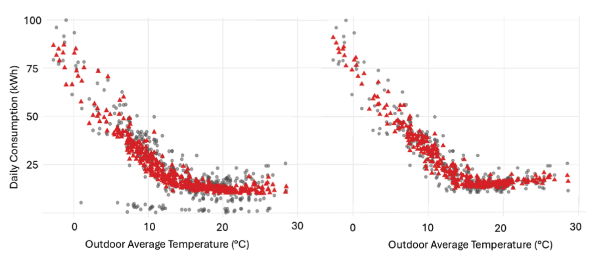
Figure 2
Example of data cleaning removing low consumption and impact on modelled values. Left: before, right: after. In red: modelled, in grey: metered values.
The explanatory variables extracted from the questionnaire include: type of housing (SFH, MFH), use of air conditioning (AC-yes, AC-no), PV equipment installed (PV-yes, PV-no), floor area (m2), number of inhabitants, Heating Degree Days (HDD), type of AAHP (multi or mono-split), type of domestic hot water (DHW) (electric, thermodynamic, solar, other), renovation work (retrofit-yes, retrofit-no).
For the clustering, we used the declared use of space heating system (as a declared percentage of use) in the pre- and post-situation: pre-k or post-k with k = (AAHP, REH, boiler, fireplace, stove).
For the energy savings model, we also used the following variable for pre/post situations: the main heating system and the space heating use (mixed, single). We added the daily electricity consumption (DC) during periods of cold outdoor temperatures (T ∈ [–1°C, 1°C]) to consider the electrical intensity of space heating linked to the winter cold.
Local normal climate – step 2
To estimate the local normal climate (step 2 of the analysis, Figure 1), we use the average daily temperature over the studied period. This daily temperature record is then smoothed using a second-harmonic Fourier series model (Duchon & Hale 2012):
where i ∈ {1, …,365} represents the calendar day.
Because spatial data were anonymized at the departmental level (French administrative division), site-specific normals were computed using three years of local weather data.
A three-year period is short compared to conventional 30-year climate records. However, a study shows that shorter periods improve representativeness and provide better balance between bias and variability to account for climate change (Ye et al. 2026).
Multivariate adaptive regression spline modelling – step 3–4
In Step 3 of the analysis (Figure 1), a non-parametric regression model based on multivariate adaptive regression splines (Friedman, 1991) is used, which combines recursive partitioning and spline fitting. We used the enhanced adaptive regression through hinges (EARTH) R package (Milborrow 2023) to model the daily consumption (DC) as a function of the outdoor temperature (Figure 3). The EARTH model performs automatic selection of predictors (explanatory variables) and the number of knots. The modelled daily consumption DC is based on the following equation 2.
where
with
DC: daily electric consumption (kWh/day) on day d.
Ti: average daily outdoor temperatures (°C) for the day d and the 2 previous days (i = 1 – 3) included to account for building thermal inertia and temporal dependence.
Wj: dummy variable indicating the day of the week (j = 1, …, 6), with the omitted category serving as the reference day.
ci: estimated knot locations of the hinge functions.
αi(+), αi(–), βi, β0: estimated model coefficients.
ɛd: residual error term.
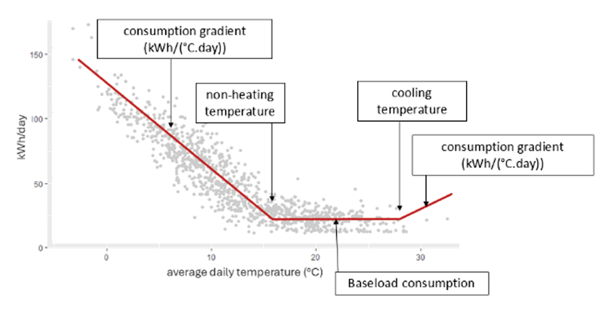
Figure 3
Schematic representation of the daily consumption gradients (all end-uses), non-heating temperature threshold and cooling temperature (tipping points) (Osso et al. 2024).
Separate models were fitted for each dwelling before and after AAHP installation (176 models in total). As demonstrated in Osso et al. (2024), algorithm selection has a minimal effect on net annual energy estimates relative to temperature-gradient fitting. Therefore, no other model types were tested.
Electricity savings evaluation – step 5
In steps 5 of the analysis, the assessed ESn (in kWh/year) for each n dwelling is calculated (equation 3) as the difference of the sum of daily consumption modelled at local normal climate in the pre- (REH) and post- (AAHP) situations for a one-year period (i = 1 to 365).
Clustering – step 6
The household clustering based on the variables of the questionnaire is performed in two steps: principal component analysis (PCA) followed by classification. PCA helps to identify the variables that produce the most homogeneous clusters. Firstly, the PCA searches for the subspace that best represents the diversity of individuals and that maximises the variance of the projected points and based on linear relationships between variables. The proximities between variables are interpreted in terms of correlation; the proximities between individuals are interpreted in terms of overall similarities in the observed values (Lebart, Morineau & Piron 1995; Husson, Josse & Pagès 2010).
We used the FAMD (factor analysis for mixed data) function which is a combination of PCA for quantitative variables and multiple correspondence analysis (MCA) for qualitative variables of the FactoMineR package (Lê, Josse, & Husson 2008).
In a second stage, to identify homogeneous individual profiles, agglomerative hierarchical clustering was performed on the coordinates of individuals from the PCA using the hierarchical clustering on principal components (HCPC) method, using the HCPC function of the FactoMineR package (Lê, Josse, & Husson 2008).
Generalized additive models for location, scale and shape – step 6
In step 6 of the analysis (Figure 1), we also modelled the ESn in kWh/year, and not the ESUn in kWh/(m².year), with the GAMLSS methodology to avoid the floor area on both sides of the equation. The objective is to quantify the impact of explanatory variables on electricity savings fluctuations.
Generalized additive models for location scale and shape (GAMLSS) are distributional regression models to overcome some limitations of generalized linear models especially when the response variable exhibits heterogeneity. They allow us to model not only the mean of a distribution, but also its variance, skewness, and kurtosis (Stasinopoulos & Rigby 2007). GAMLSS models use a distributional regression approach in which all parameters of the conditional distribution of the response variable are modelled using explanatory variables with four parameters:
Mean (µ). Models the mean of the response variable (location).
Variance (σ). Characterizes the dispersion or variability of data (scale).
Skewness (υ). Measure of a distributional asymmetry with a skewness of zero in case of a symmetric distribution (shape).
Kurtosis (τ). Measure the heaviness of the tail in a distribution compared to the normal distribution (shape).
For each parameter θk (with θ ϵ {μ, σ, υ, τ}), named as the distribution parameters, the GAMLSS model defines a relationship such as eq. 4 (Stasinopoulos & Rigby, 2007).
with: gk(.) the link function for each parameter, Xk βk the linear effects, the smoothing function.
Using the R package gamlss (Stasinopoulos & Rigby 2007), the first step to build the model is the selection of the best non-Gaussian distribution with a simple model without explanatory variables using the Generalized Akaike Information Criterion (GAIC). The second step is the selection of explanatory variables and the type of relationship (linear, spline …).
Results
Electric daily consumption modelling
The EARTH models successfully captured temperature dependencies in both pre- and post-retrofit periods. No change point detection method for determining non-routine events was used.
Figure 4 shows an example of daily consumption pre- and post-situation in the observed period based on the average outdoor temperature. It should be noted that, overall, the EARTH model manages to capture the impact of the outdoor temperature despite significant variations in consumption at a fixed temperature.
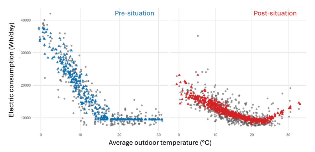
Figure 4
Example of daily consumption modelling pre- and post-situation of AAHP installation. Left blue: pre-modelled, right red: post-modelled, in grey: metered values.
The goodness-of-fit (R²) by the models is presented in Figure 5 for the 88 households in pre- and post- situations. A higher R² means the model better explains consumption using our available variables. The unexplained variation is treated as the residuals.
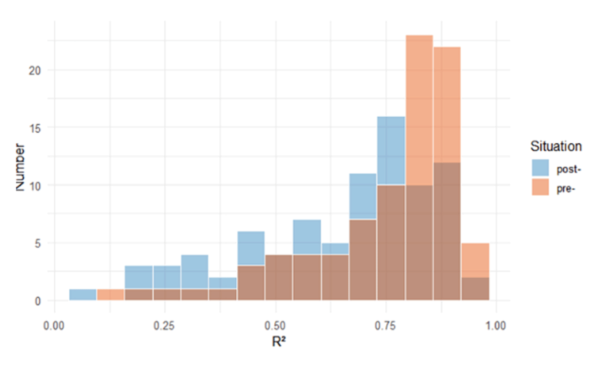
Figure 5
Histogram of the coefficient of determination (R²) of the EARTH models in pre- and post-situation. R² mean: pre- = 0.749, post- = 0.652.
The median coefficient of determination (R²) of all the EARTH models is respectively 0.8 and 0.71 for the pre- and post-situation. The lower post-retrofit R² reflects lower thermal sensitivity following AAHP adoption, which increases the relative impact of variations in consumption that act as noise with respect to the model. This suggests that the higher the R², the greater the REH consumption and thus the higher the resulting ES. This assumption will be used in the ES GAMLSS model as a potential explanatory variable (i.e. DC with T ∈ [–1°C; 1°C]). For the clustering we used directly the R² of the EARTH model in the pre- and post-situation as an additional variable (pre-R², post-R²).
Evolution of baseload consumption
In the absence of a control group, to check for baseline consumption shifts unrelated to space heating, annual consumption during mild weather periods (16°C ≤ T ≤ 20°C) was compared from pre- to post- situations (see Figure 4 and Figure 6 as examples).
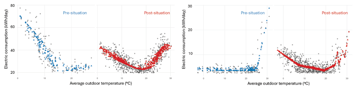
Figure 6
Examples of new uses (left) for air conditioning in the post-situation (red) and pre-existing air conditioning (right) in the pre-situation (blue).
This consumption remains virtually stable, displaying a negligible mean change of –22 kWh/year (median = –24 kWh/year, Q1 = –90 kWh/year, Q3 = 60 kWh/year).
Air-conditioning assessment
Most respondents reported using AAHPs for summer cooling after installation (AC-yes = 87%). However, some households already had air conditioning, as shown in Figure 6, with a daily consumption gradient for the hottest days in the pre-situation (and without REH).
To evaluate the use of air conditioning associated with the installation of a reversible AAHP, we calculate the difference in annual consumption when the average daily temperature is above 16 °C. It should be noted that this temperature level may seem low, but it should be borne in mind that this is the daily average value. However, daily minimum and maximum temperatures were unavailable, although the daily maximum temperature would have been a more suitable variable. Ademe and Enertech (2025) also notes a daily average temperature of between 15 and 16 °C associated with the start of air conditioning use.
The increase in consumption during hot periods is approximately 1.1 kWh/m² on average (median 0.54 kWh/m²), with significant variations (Figure 7).
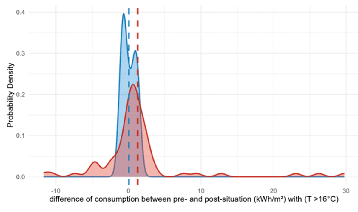
Figure 7
Distribution showing the increase in consumption (in kWh/m²) between the pre- and post-situations, with an average daily outdoor temperature above 16°C, based on the respondent’s reported use of air-conditioning (AC-yes in red, AC-no in blue). Dashed lines = mean value.
If households are divided into two groups, those who report using air conditioning (AC-yes) and those who do not (AC-no), the average new consumption is 1.27 kWh/m² (s.d. = 6.25) and 0.06 kWh/m² (s.d. = 0.88) respectively. This difference is non-significant (Welch Two Sample t-test, p-value = 0.12) (Delacre, Lakens & Leys 2017). This could be explained by the high variance within the “AC-yes” group and bimodal behaviour in the “AC-no” group.
A possible explanation is that some households may well have used their appliances on automatic mode or may have underestimated their air-conditioning consumption. One way to verify this is to look at the temperature gradients for hot days, but the wide variation in consumption during these periods poses a problem. Ideally, an additional summer of data would be required, as this was the first summer during which many users operated air conditioning following the installation of the AAHP. Consequently, user adaptation remains incomplete, and the corresponding utility bill has not yet been received. This represents a potential improvement for future research.
Electricity savings assessment
The ESU assessment based on the difference in annual electricity consumption modelled by the EARTH model averages 14.6 kWh/m² (median = 13.5 kWh/m²) with a significant deviation (Q1 = 4.0 kWh/m² and Q3 = 22.0 kWh/m²) (Figure 8). This ESU corresponds to an absolute value of an average ES of 1,630 kWh/year for a modelled pre-consumption of 9,400 kWh/year for all electric end-uses.
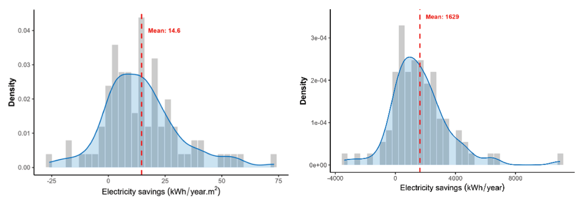
Figure 8
Histogram of the assessed electricity savings (left: ESU in kWh/(m².year)), (right: ES in kWh/year). All end-uses electricity savings including air-conditioning and gas boiler to AAHP switch (i.e. negative savings).
We observed a minimum ESU value of -26 kWh/(m².year) and a maximum value of 73 kWh/(m².year). The large negative values are those related to the use of a gas boiler in the pre-situation.
Households clustering
FAMD reduced survey dimensions with the first five axes accounting for 63.2% of cumulative sample variance (see Annex). The first two dimensions of the FAMD account for 17.6% and 14.8% of data variability respectively (Figure 9 and Table 3 in Annex).
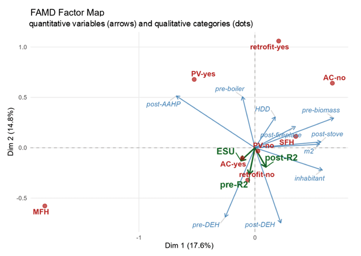
Figure 9
Visualisation of the correlation coefficients between variables and the principal components (the first two axes). In blue: quantitative variable, in red: qualitative variables, in green: additional variables. The quantitative variables are represented as arrows on these axes: the longer the arrow and the closer it is to an axis, the more closely the variable is linked to that axis. Categorical variables are represented by dots: two categories that are close to each other in the space indicate similar profiles in the data. ESU, R² are included as illustrative variables.
The electricity savings per unit area (ESU in kWh/m²) are positively correlated with the pre- and post-REH uses as declared by the household. The savings are negatively correlated with the gas boiler used and the heating degree day (HDD). The household size and the floor space are lightly correlated with the ESU.
Notably, the performance of the model (i.e. the level of explanation of the variance of the daily consumption, as expressed by the R²) is correlated with the ESU and the use of REH in the pre-situation (correlation coefficient of 0.3). This could be explained by the fact that the higher the temperature gradient during cold days (i.e. daily consumption depends largely on consumption related to space heating), the higher the explanation of variance by the EARTH model (higher R²) and the higher are the potential ESU.
In summary, the first dimension (Dim 1) differentiates housing types (MFH vs. SFH) and biomass use. The second dimension (Dim 2) differentiates retrofit and AAHP use vs. direct electric heating use. Renovated buildings with heat pumps use and PV panels cluster in the upper-left quadrant, opposing non-retrofitted, REH use in the lower-left/bottom. SFHs correlate with wood-based heating use and larger living spaces, positioned opposite MFHs.
The HCPC analysis identified four distinct household clusters (Figure 10) which are mainly characterized by the following variables (see Tables 4 and 5 in Annex):
Cluster 1 (n=13): MFH with high REH (100% vs. mean: 85.5%) and low floor area (75 m² vs. mean: 115 m²). Mean ESU = 10.1 kWh/m² (median = 4.8 kWh/m²).
Cluster 2 (n=2): gas boiler use (100% vs. mean: 2.35%) and no REH use, and high HDD (2,908 vs. a mean of 1,938). Mean ESU = –17.6 kWh/m² (median = –17.6 kWh/m²).
Cluster 3 (n=66): SFH with large floor area (125 m² vs. mean: 115 m²) and higher use of AAHP in the post-situation (87.5% vs. mean: 85.2%). Mean ESU = 16.5 kWh/m² (median = 13.9 kWh/m²).
Cluster 4 (n=5): high use of biomass space heating in the pre-situation (30.6% vs. mean: 5.2%) and in the post-situation (27.0% vs. mean: 2.6% for wood stove and 10% vs. mean: 1.66% for fireplace). Low AAHP use (42% vs. mean: 85.2%) and higher household size (3.4 vs. mean: 2.4). Mean ESU = 14.6 kWh/m² (median = 14.2 kWh/m²).
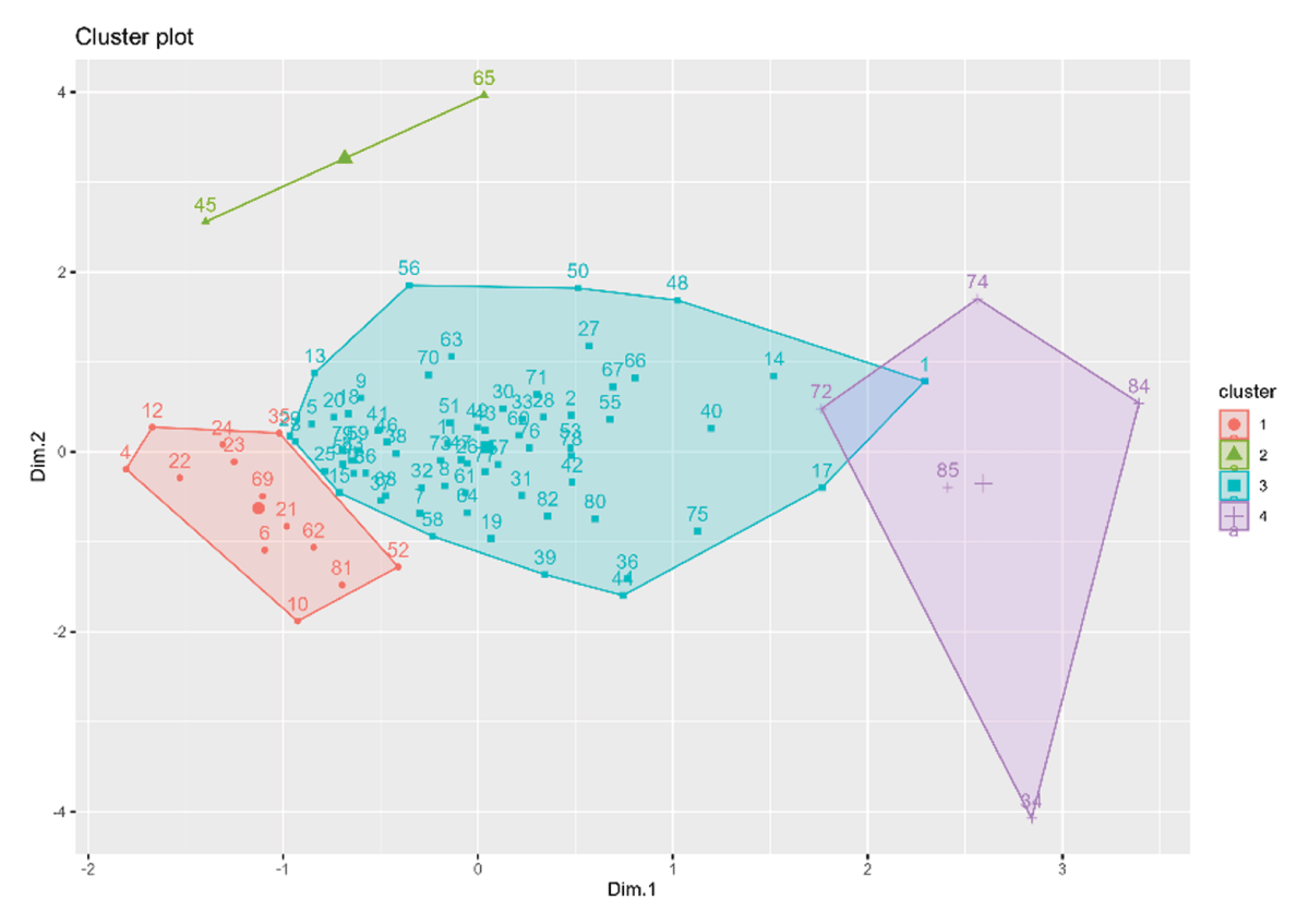
Figure 10
Cluster visualization (HCPC) in the FAMD map (the first two axes). Projection of individuals onto the first two dimensions of the FAMD. Observations are grouped into four clusters identified via Hierarchical Clustering on Principal Components (HCPC). Proximity: Points located close to each other represent individuals with similar characteristics or survey responses. The two main axes (Dim 1 & Dim 2) summarize most of the variation in the dataset (see Figure 9).
We note that Cluster 2, containing only two individuals, together with observation 34 in Cluster 4, may be interpreted as outlying observations.
In Figure 10, the horizontal axis (Dim 1 of the FAMD analysis – see Figure 9) highlights the main contrast between Cluster 4 (right) and the others. The vertical axis (Dim 2) sets Cluster 2 (top) apart from the rest. Located on the left side, Cluster 1 brings together individuals with lower or negative values on Dimension 1. Cluster 2 is a small, distinct group at the top left, characterized by particularly high values on Dimension 2. Cluster 3 is the largest and most central group, representing the average profile of the majority of observations. Positioned on the far right, Cluster 4 gathers unique profiles that differ significantly from the rest along Dimension 1.
A global Kruskal-Wallis test4 (Kruskal & Wallis 1952) revealed a significant difference in ESU between all clusters (p = 0.038) (Figure 11). Post hoc comparisons using Dunn’s test5 (Dunn 1961) confirmed that this difference was driven solely by Cluster 2 (gas boiler use) (p = 0.0456). Savings differences among Clusters 1, 3, and 4 were not statistically significant.
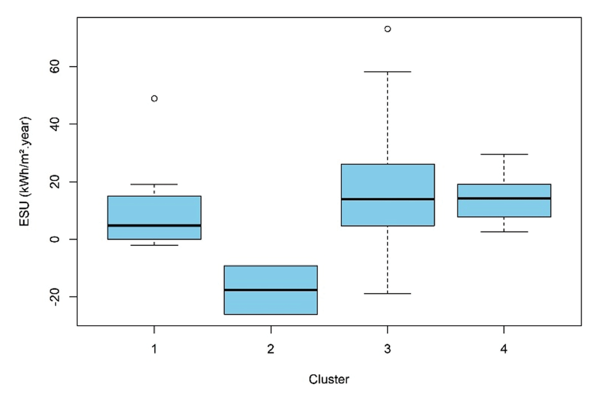
Figure 11
Boxplot of electricity savings (ESU in kWh/(m².year)) per HCPC cluster.
As clustering struggles to identify differences in electricity savings, apart from households that previously used a gas boiler, we propose modelling savings without Cluster 2 and based on a set of variables, as presented in the following section.
Energy savings modelling
Absolute annual electricity savings (ES in kWh/year) were modelled using GAMLSS by excluding Cluster 2 (use of gas boiler by only 2 respondents) from the panel. A type 3 Skew T distribution (Fernández & Steel, 1998) was selected according to the generalised Akaike information criterion (GAIC) using the automated distribution selection function (chooseDist) of the gamlss package which analyzes a large distribution set. The AIC is a metric used to compare different models for the same dataset, balancing the goodness of fit against the complexity of the model.
Few variables are significant to explain ES (Table 2), only the household size and the daily consumption in cold weather (µ parameter). Furthermore, the variance (σ) depends on the surface area and the daily consumption in cold weather. The shape parameters show that the distribution is symmetric (skewness (υ) non-significant and close to zero) but with a heavy tail (as kurtosis (τ) is significant) showing extreme values (outliers). The prediction errors of the model are normally distributed and that there is no systematic bias hidden in the quantile residuals (see the wormplot in Figure 14 in Annex).
Table 2
GAMLSS model of the annual electricity savings (ES in kWh/year). Explanatory variables are normalised.
| ESTIMATE | STD. ERROR | t-VALUE | p-VALUE | |||
|---|---|---|---|---|---|---|
| µ coefficients(mean) | (Intercept) | 1699.0 | 306.0 | 5.553 | 4.18e–07 | *** |
| Household size (unit) | –328.5 | 112.5 | –2.918 | 0.00466 | *** | |
| Daily consumption during cold days (T = [–1°C, 1°C]) (kWh/day) – pre-situation | 975.7 | 196.7 | 4.959 | 4.37e–06 | *** | |
| σ coefficients(variance) | (Intercept) | 6.9206 | 0.1491 | 46.428 | <2e–16 | *** |
| Daily consumption during cold days (T = [–1 °C, 1 °C]) (kWh/day) – pre-situation | 0.3451 | 0.1307 | 2.641 | 0.0101 | * | |
| Floor area (m²) | 0.2629 | 0.1364 | 1.928 | 0.0576 | . | |
| υ (skewness) | (Intercept) | –0.008775 | 0.15704 | –0.056 | 0.956 | |
| τ (kurtosis) | (Intercept) | 1.5300 | 0.57773 | 2.65 | 0.00983 | ** |
[i] Only significant variables are presented, others as presented in Table 1, are not significant or collinear with the selected variables (see Table 13 in Annex).
Note: *p < 0.05, **p < 0.01, ***p < 0.001.
No. of observations in the fit: 83 – Degrees of Freedom for the fit: 9.
Residual Deg. of Freedom: 74 – Global Deviance: 1,421.897 – AIC: 1,439.897 – SBC: 1,461.666.
The Nagelkerke’s6 Pseudo-R² (Nagelkerke 1991), reaches 0.437, indicating that the model explains nearly 44% of the variance in ES. The simple coefficient of determination (R² = 0.377) indicates that the structure of the mean (µ) explains only 38% of the variance in consumption. This means that most of the variance in ES remains unexplained by the variables at our disposal.
Translating normalised effects in absolute values indicates that (Figure 12):
One additional unit of consumption (+1 kWh/day) at outdoor average temperature between [–1°C, 1°C] changes the ES by: +35 kWh/year;
and one additional occupant reduces ES by: –306 kWh/year.
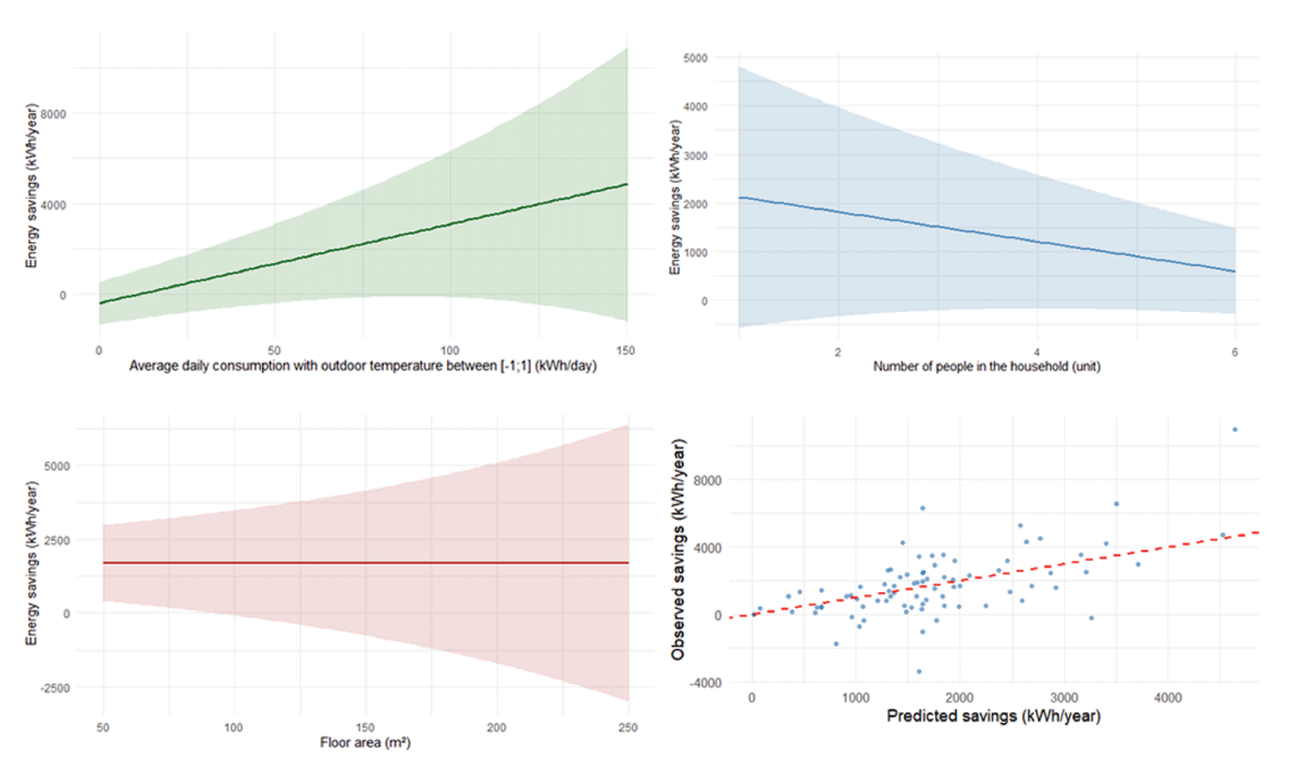
Figure 12
Marginal effect of explanatory variables on the predicted mean (µ), with a 95% prediction interval incorporating the dispersion parameter (σ). Bottom right: observed values versus predicted values, red dashed line: perfect fit.
Households that consume more energy during cold days in the pre-situation achieve significantly higher energy savings per year. Larger households tend to achieve slightly lower energy savings per year compared to smaller households. The size of the home does not appear to influence annual energy savings directly, though uncertainty (the shaded area) increases for larger homes.
Discussion and conclusion
This study developed a climate-adaptable model, based on multivariate adaptive regression splines, which can assess electricity savings when changing the space heating equipment from REH to AAHP. Unlike earlier estimates (Dupret 2025), our approach avoids assuming complete substitution of secondary heating systems. This study evaluates real-world energy savings beyond the theoretical or nominal efficiency of AAHPs.
A key challenge in evaluating field performance is the high variability in occupant behaviour, which cannot be fully captured by standard survey questionnaires. Furthermore, there is a discrepancy between ‘idealized’ self-reported behaviour and actual reality.
We were also limited by the available data (only average daily outdoor temperature), without maximum daily temperature or wind speed which were identified in a previous paper (Osso et al. 2024) as important explanatory variables. However, the lack of this data does not prevent us from drawing some conclusions.
To address these questions, we first modelled pre- and post-situation electricity consumption under local normal climate conditions using daily smart meter data. Secondly, we estimated the energy savings for each dwelling. Finally, we attempted to explain the variations in these energy savings using survey data.
Even with a relatively large sample based on smart meter data and field surveys, drawing clear conclusions remains challenging. Although our model explained ~44% of the variance in annual electricity savings (Nagelkerke R²), a large share of individual savings variability remains unexplained. This does not mean that this unexplained variance could not potentially be explained with additional information. In any case, there will always be an unexplainable portion driven by the underlying complexity, context, and intrinsic randomness of real-world phenomena.
The clustering of households clearly identifies four different clusters with specific characteristics, but whose electricity savings differences are not statistically significant, except for one group that used a gas boiler before the AAHP was installed. Once again, the diversity of situations makes it difficult to measure differences that may not be so great within large variations.
It remains difficult to explain the variations in ES, as the variations in daily consumption are significant. Consequently, larger household size is associated with lower electricity savings, whereas higher initial consumption during cold weather. (i.e. a high dependence of daily consumption on outdoor temperature) leads to greater savings. This variable likely captures the combined effects of the initial heating systems (e.g. REH in combination with biomass heating) as well as the building’s insulation level. This explains why the declarations of intensity of use of supplementary to REH heating are not significant. Consistent with expectations, the higher the previous electricity consumption, the greater the electricity savings will be. This also highlights the impact of secondary heating (e.g. biomass) on the savings that can be expected with the installation of AAHP.
It should be noted that floor space has no effect on the average ES, but only on the variance, which increases with floor space. The diversity of occupations may increase with the space available. Since the size of the household is correlated with floor area (Figure 13 in Annex), the model retains the most relevant variable. However, variables such as additional retrofit or the presence of PV are not statistically significant, probably due to the lack of representative households (20 and 4 households respectively in the dataset). A larger sample for these scenarios could allow the effects to be estimated.
Regarding summer cooling, although most households reported using AAHPs for space cooling, the associated energy consumption was minimal (averaging < 1.3 kWh/(m²·year)) and did not offset winter heating savings. Consequently, the net energy balance remains positive, confirming that summer cooling demand remains secondary to space heating savings. The difference in cooling consumption between households reporting AC use and those who do not is statistically non-significant. This is understandable, as according to a survey, few households use it all day long (16%) and 54% use it only during heat waves and 10% never use it (ADEME 2025). A wide variety of occupant behaviours: between rooms in the same dwelling, from one day to the next, and between different dwellings has already been documented (CSTB 2025). Thus, variations in air-conditioning use associated with low consumption make it difficult to estimate the consumption. This estimated cooling consumption could serve to support the EEO valorisation for the AAHP standardized operation sheet in case of revision.
Despite the energy savings, AAHPs do not benefit from the support of all aid schemes because their reversible nature seems to be an obstacle to incentives, so as not to encourage the development of air conditioning. At the time of writing, the AAHP is not eligible for the reduced VAT rate (5.5% vs. 20%) applicable to other heating equipment such as AWHPs or boilers (Bofip 2014) nor subsidized aid from the EEO scheme (“Coup de pouce”) (MTE 2025), nor state incentives such as “Ma Prime Rénov’” (ANAH 2025). However, adapting to climate change requires the use of both passive solutions, such as external shading, and active solutions, such as air conditioning (Viguié et al. 2020). This study helps demonstrate the relevance of AAHPs for the electrification and decarbonisation of residential space heating as well as a moderate use of air conditioning.
The insights provided by this study can inform policy makers and, most importantly, feed into studies on energy savings potential. This study may also be used to investigate the impacts of the increasing deployment of heat pumps on the electricity load curve.
For future studies of this kind, additional questions could be included to improve the explanatory quality of energy savings variation analyses. Notable additions could include daily temperature extremes, beyond average temperatures, and the dwelling’s energy performance certificate rating.
Disclaimer
The information and views set out in this study are those of the authors and do not necessarily reflect the official opinion of their affiliation.
Appendices
Annex
Correlation matrix
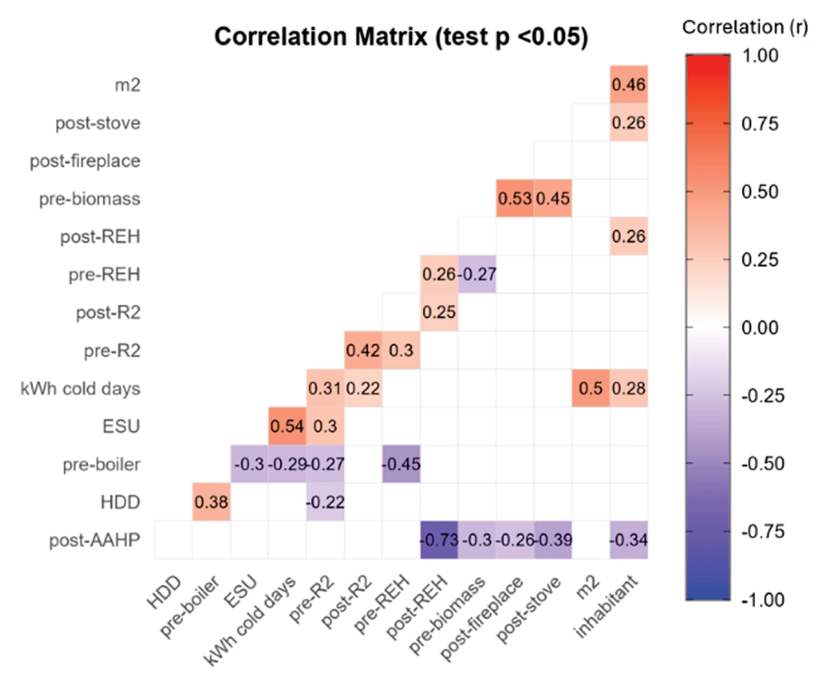
Figure 13
Correlation matrix between the variables studied. Only statistically significant correlations at the threshold are displayed. The empty spaces correspond to non-significant coefficients (p ≥ 0.05).
Hierarchical clustering on principal components
Table 4
Characterization of clusters resulting from hierarchical ascending classification on principal components (HCPC).
| DISCRIMINANT QUANTITATIVE VARIABLES (v-TEST) | ||||||
|---|---|---|---|---|---|---|
| VARIABLE | v.TEST | MEAN IN CATEGORY | OVERALL MEAN | SD IN CATEGORY | OVERALL SD | p.VALUE |
| Cluster#1 | ||||||
| pre-REH | 2.006 | 100 | 85.05 | 0.00 | 28.967 | 4.476451e–02 |
| m² | 3.921 | 75 | 115.67 | 18.518 | 40.358 | 8.813829e–05 |
| Cluster#2 | ||||||
| Pre-boiler | 9.218 | 100.00 | 2.348 | 0.00 | 15.069 | 3.009722e–20 |
| HDD | 3.513 | 2908.4 | 1937.91 | 1074.4 | 392.90 | 4.414451e–04 |
| pre-R² | –2.486 | 0.464 | 0.756 | 0.341 | 0.167 | 1.291103e–02 |
| ESU | –2.719 | –17.611 | 14.647 | 8.443 | 16.872 | 6.528922e–03 |
| pre-REH | 4.177 | 0.00 | 85.05 | 0.00 | 28.967 | 2.950168e–05 |
| Cluster#3 | ||||||
| m² | 3.568 | 124.272 | 115.67 | 39.936 | 40.358 | 0.0003594492 |
| post-AAHP | 2.393 | 87.454 | 85.139 | 10.812 | 16.197 | 0.0166776343 |
| post-stove | –2.295 | 1.363 | 2.616 | 4.650 | 9.141 | 0.0217311903 |
| pre-boiler | 2.576 | 0.030 | 2.348 | 0.244 | 15.069 | 0.0099715353 |
| Cluster#4 | ||||||
| post-stove | 6.110 | 27.0 | 2.616 | 22.715 | 9.141 | 9.957710e–10 |
| pre-biomass | 4.804 | 30.6 | 5.209 | 18.039 | 12.104 | 1.548102e–06 |
| post-fireplace | 2.952 | 10.0 | 1.662 | 20.00 | 6.467 | 3.148761e–03 |
| inhabitant | 2.223 | 3.4 | 2.371 | 1.743 | 1.059 | 2.619405e–02 |
| post-AAHP | 6.100 | 42.0 | 85.139 | 21.354 | 16.197 | 1.055582e–09 |
[i] The mean in category indicates the average value within the cluster, compared to the overall mean of the sample. The clusters were characterized using the v-test. A variable is considered characteristic of a cluster if the difference between its intraclass mean and its overall mean is statistically significant, which corresponds to a |v-test| ≥ 1.96 (equivalent to a threshold of p < 0.05).
Table 5
Characterization of clusters by qualitative variables (HCPC).
| DISCRIMINATING QUALITATIVE CRITERIA (v-TEST) | |||||
|---|---|---|---|---|---|
| CATEGORY | CLA/MOD | MOD/CLA | GLOBAL | p.VALUE | v.TEST |
| Cluster#1 | |||||
| MFH | 92.857 | 100 | 16.279 | 1.608517e–14 | 7.678588 |
| SFH | 0.000 | 0 | 83.720 | 1.608517e–14 | –7.678588 |
| Cluster#2 | |||||
| Non significant | |||||
| Cluster#3 | |||||
| SFH | 91.666 | 100 | 83.720 | 8.540566e–12 | 6.829173 |
| MFH | 0.000 | 0 | 16.279 | 8.540566e–12 | –6.829173 |
| Cluster#4 | |||||
| Nonsignificant | |||||
[i] Cla/Mod (Percentage of the Cluster in the Category): Proportion of individuals with this category in the cluster (measure of specificity). Mod/Cla (Percentage of the Category in the Cluster): Proportion of individuals in the cluster with this category (measure of representativeness). Global: Relative frequency of the category in the entire sample. v-test Standardized score, a|v-test| ≥ 1.96 indicates a statistically significant representation of the category within the cluster compared to the overall average.
Wormplot of the residuals of the GAMLSS model
The adequacy of the model was assessed using the Shapiro-Wilk normality test (p-value = 0.9959), demonstrating that prediction errors are normally distributed and that there is no systematic bias hidden in the quantile residuals:
Mean (–0.003): Very close to zero, the model neither overestimates nor underestimates consumption overall.
Variance (1.01): Very close to 1, target for standardised residuals.
Skewness (0.02): Very close to zero, errors are symmetrical.
Kurtosis (2.84): Close to 3 (the normal value), few extreme outliers that the model would not have been able to handle.
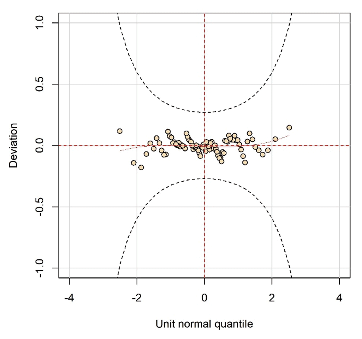
Figure 14
Worm plot (van Buuren & Fredriks 2001) of the normalised quantile residuals for the GAMLSS model. The Deviation axis represents the difference between the observed and theoretical quantiles. The horizontal elliptical curves represent the 95% confidence limits. The flat shape of the red trend line and the inclusion of all residuals within the confidence bands indicate an adequate model fit, capturing the location, scale, and shape parameters of the response variable distribution.
Notes
[4] This carbon content is based on the smoothing of data from 2024, 2023, 2022, and 2021. The upstream includes: fuel upstream, power plant depreciation, and ancillary operating emissions (ADEME 2024).
[5] Joule stated the relationship between the current flowing through a resistor and the heat dissipated by it, since known as Joule’s law (Wikipedia).
[6] In a work published in 1824, Carnot laid the foundations for an entirely new discipline: thermodynamics (Wikipedia).
[7] ‘The Kruskal-Wallis is a nonparametric statistical test that assesses the differences among three or more independently sampled groups on a single, non-normally distributed continuous variable.’ (McKight & Najab 2010).
[8] ‘Dunn’s test is the appropriate nonparametric pairwise multiple comparison procedure when a Kruskal–Wallis test is rejected’ (Dinno 2015).
Acknowledgements
C. Laruelle and J. Louis from the French Agency for Ecological Transition (ADEME) for providing the survey data in the framework of the COPACAIR research project. L. Xiao (EDF) for her support in carrying out this study.
Data Accessibility Statement
The dataset analyzed in this study is publicly available on the ADEME data platform at https://data.ademe.fr/datasets/pac-campagne-de-mesure-rr.