
1 Introduction
The transition to a decarbonised energy system requires the mass adoption of Low-Carbon Technologies (LCTs) by domestic consumers, primarily Photovoltaics (PV), Electric Vehicles (EVs) and Heat Pumps (HPs). As these technologies shift energy loads from fossil fuel networks to the electricity grid, the magnitude and timing of peak demand are expected to change significantly (Damianakis, Mouli and Bauer, 2025).
Unlike Scandinavian countries such as Norway, Sweden and Finland, which have historically relied on electrified heating underpinned by abundant hydro and nuclear generation capacity (Satymov et al., 2025), the UK’s residential heating system is predominantly gas-based, with approximately 85% of homes connected to the gas network (Gillich, 2025). This gas dependency is the critical structural difference driving the electrification challenge: where historically all residential thermal demand was met by combustion at the point of use, requiring only low-voltage electricity for controls and appliances, the transition to HPs transfers this large, synchronised heating load directly onto the electricity grid. This is not simply an issue of fuel substitution; it is a fundamental rebalancing of the energy system’s physical infrastructure requirements.
This creates a fundamentally different electrification challenge: the UK electricity grid and its distribution infrastructure were not designed to carry the synchronised peak loads that mass heat pump and EV adoption will generate during winter evenings. Addressing this gap requires large-scale empirical evidence from real UK housing stock, rather than models derived from non-analogous international contexts. While this paper focuses on the UK context, the transition from gas to electric heating is an active challenge across many gas-dependent European economies, including Germany, the Netherlands, Belgium, and Ireland, and the empirical methodology and peak-demand findings presented here are therefore of direct relevance to researchers and network planners in those regions (Damianakis et al., 2023; Damianakis, Mouli and Bauer, 2025).
Most existing assessments of LCT impacts rely on synthetic load profiles or small-scale trials. There is a critical need for large-scale empirical evidence that accounts for the diversity of the UK housing stock (McKenna et al., 2016; Damianakis et al., 2023; Evans et al., 2023). To isolate building performance from dwelling size, this study uses peak Power Density (W/m2). Larger homes naturally draw higher absolute loads, which can mask the underlying efficiency of the building-technology system. By normalising demand and stratifying households by insulation level and housing type, this research attempts to identify how building fabric, rather than just house size, could be driving peak electrical demand.
The paper proceeds as follows: Section 2 details the EUI normalisation methodology and statistical approach; Section 3 describes the SERL dataset, quality control, and cohort classification; Section 4 presents results by technology group; Section 5 discusses implications; Section 6 outlines limitations; and Section 7 draws conclusions.
1.1 Literature review
The transition to a net-zero residential sector relies on the ‘electrification of everything,’ yet the resulting surge in peak demand creates significant challenges for existing infrastructure (Millar et al., 2025). This shift requires a deeper understanding of how building fabric, building services and appliances, and occupant practices converge to strain the electricity grid during winter peaks.
Current scholarship identifies a widening ‘performance gap’ between theoretical models and empirical reality. Few et al. (2023) demonstrate a critical “performance gap” where EPC models systematically over-predict primary energy use as building efficiency declines. While bands A and B align with metered data, the model over-predicts intensity by 8% for band C and 48% for bands F and G. Crucially, this discrepancy persists even when controlling for normative occupancy and heating set-points (21°C), suggesting that the gap is not purely behavioural but a structural limitation of the SAP model (SAP: Standard Assessment Procedure; the UK’s official methodology for calculating a dwelling’s energy performance and carbon emissions). The reliance on pessimistic default values for uninsulated fabrics creates a theoretical demand divorced from the “As-Operated” reality.
This evidence explains the inverse relationship observed in this study: “leaky” homes exhibit lower-than-predicted peaks because their theoretical benchmarks are fundamentally inflated. This confirms that standardised models fail to capture the non-linear relationship between building physics and empirical grid impact.
1.1.1 Case study: the EUI framework in large-scale urban analysis
An application of the EUI framework is found in a study (Liddiard et al., 2021) that utilised a longitudinal study of over 1.2 million London-based dwellings to demonstrate the limitations of absolute consumption metrics. By normalising energy data into kWh/m2 and W/m2, their research successfully decoupled the physical scale of a dwelling from its operational efficiency. The study highlighted a significant “performance gap” in existing assessment models; while building size was confirmed as the primary determinant of gross energy, the correlation between actual normalised demand and asset-based EPC ratings was surprisingly weak. This is partly due to the structural logic of the domestic EPC, which functions as a cost-based index rather than a direct measure of thermal or energy efficiency. Consequently, its ability to predict peak electrical demand is fundamentally limited, particularly in electrified homes where high unit costs for electricity can skew the rating regardless of the building’s physical performance.
1.1.2 Heat pumps at evening peak
The deployment of HPs is expected to cause a significant shift in domestic load profiles. Empirical evidence from Oxford University using SERL (Agrawal and Wallom, 2026) shows that switching from mains gas heating to air source HP fundamentally reshapes the evening load, with full deployment more than doubling winter evening peaks from a 68 kWh baseline to 149.7 kWh at the substation level. For a detached dwelling, this represents an absolute demand of approximately 3.1 kW (or 25.8 W/m2). This intensification is “front-loaded,” with detached homes driving disproportionate grid stress during early adoption, creating immediate “hotspots” that threaten the capacity of local low-voltage transformers.
A critical counter-narrative is provided by Bernard et al. (2024) in their large-scale evaluation of the ‘Cosy’ Time-of-Use (ToU) tariff, a self-selected sample. They found that smart pricing signals lead to a near-doubling of consumption during off-peak windows and a halving of consumption during the evening peak. Crucially, they found that this load-shifting behaviour did not diminish on the coldest days; in fact, the absolute magnitude of shifted load was higher during extreme cold, as there was more total heating demand available to be flexible. This confirms that building insulation is not the sole determinant of grid resilience; when paired with price signals, occupants can leverage a building’s thermal mass to “pre-heat,” successfully insulating the grid from the 17:00–21:00 stress window. This growing capacity for flexibility is further evidenced by Burger and Rosenow (2025), who highlight a threefold increase in adoption of European smart tariffs designed to optimise such pre-heating strategies for both HPs and EVs.
1.1.3 Technology stacking: EVs, PV, and battery integration
The “stacking” of multiple LCTs introduces complex interactions. While Electric Vehicle (EV) charging is a high-magnitude load, it is increasingly governed by smart charging regulations (UK Gov, 2021) and time of use tariffs, which incentivise load-shifting away from the peak window. Recent evidence demonstrates that smart charging uptake is growing rapidly, with intelligent chargers now capable of automated off-peak scheduling that responds to both price signals and grid frequency (Acharige et al., 2025; Shariatzadeh, Lopes and Henggeler Antunes, 2025).
In summer, Solar Photovoltaics (PV) and Battery Energy Storage Systems (BESS) are identified as the primary peak-shaving assets, yet their impact is governed by complex technical and socio-technical variables. Empirical evidence from Qiu et al. (2022), utilising longitudinal smart meter data, confirms that adding battery storage to existing PV systems significantly increases the self-consumption of solar energy while reducing the volume of electricity exported back to the grid. Their study demonstrates that BESS adoption effectively flattens load curves by reducing grid reliance during system peak hours, specifically late afternoons and early evenings. However, the efficacy of these assets during winter “cold spells” is less certain. The peak-shaving potential of a BESS depends heavily on the State of Charge (SoC) and the specific control logic available; during periods of low solar yield, a battery may have insufficient energy to mitigate an evening peak unless it is also capable of grid-charging during off-peak windows.
However, Hardman et al highlight a “large degree of heterogeneity” in these patterns; in many cases, battery discharge profiles did not align with engineering or economic optimisation, such as failing to maximise discharge during peak time of use windows. This suggests that while BESS has the physical capacity to reduce peak Power Density (W/m2), the actual grid impact is highly conditional. To derive general insights into grid resilience, modelling must transition from assuming “ideal” hardware performance to accounting for the settled operational reality of these systems. Providing scalable projections for infrastructure planning requires a methodology that distinguishes stable, long-term technological performance from the transient noise of initial adoption, inconsistent control logic, or diverse occupant priorities.
1.1.4 Socio-technical drivers: self-rationing vs. comfort-taking
A critical, often overlooked dimension of peak demand is the behavioural response to energy costs and building quality. Studies on the Cost-of-Living Crisis (2022–2024) have highlighted “self-rationing”, a phenomenon where occupants in thermally disadvantaged (uninsulated) homes drastically curtail usage to avoid unaffordable bills (Zapata-Webborn et al., 2024; Singh, 2026). This behaviour creates a “statistical paradox”: uninsulated homes may appear more “efficient” in raw data (yielding a lower W/m2 peak) because their occupants are living in fuel poverty and suppressing demand. Conversely, “comfort-taking” can be observed in highly insulated homes. As demonstrated by Sunikka-Blank and Galvin (2012), the improved efficiency of the building fabric often leads occupants to maintain higher baseline internal temperatures (>21°C) for longer periods. This is driven by both the physical ability of the structure to retain heat and a behavioural “comfort-taking” effect. However, the consistency of this load is ultimately contingent on occupant demographics; while higher-income households in well-insulated homes may exhibit a stable, elevated baseline during the evening peak, lower-income cohorts may still prioritise cost-containment, albeit with a higher level of “free” warmth provided by the fabric. Conversely, in uninsulated homes, the grid impact is defined by “economic rationing,” where occupants, regardless of preference, are forced to drastically curtail usage to manage costs.
1.1.5 The research gap
While existing studies (Few et al., 2023; Agrawal and Wallom, 2026) have identified the performance gap and the macro-level impact of heat pumps on substations, there is a lack of high-resolution, empirical research that simultaneously accounts for technology stacking (the combined impact of HP, EV, and BESS) and behavioural responses across varied building fabrics. Current models either focus on single technologies or rely on “As-Prescribed” data that Few et al. have proved to be inflated. There is a gap in using metered, normalised Energy Use Intensity (EUI) to observe the “As-Operated” reality of complex, multi-technology LCT households and comparing them with control gas-heated homes, especially how this impacts upon peak evening demand.
1.2 The electrification question
The primary objective of this study is to quantify the shift in residential power density resulting from the electrification of heat and transport. Using the Energy Use Intensity (EUI) framework as a normalising lens, this research isolates the infrastructure signatures of various technology-fabric cohorts to address the following question:
“How does the integration of heat pumps and electric vehicles affect peak electrical power density (W/m2), and to what extent does building insulation or technology stacking (PV and storage) mitigate this intensification?”
2 Methodology
2.1 Normalisation and the EUI framework
Residential energy analysis often relies on absolute consumption (kWh), which introduces significant bias due to the high correlation between dwelling volume and energy demand. To mitigate this, this study utilises Power Density (W/m2) as the primary unit of observation.
By converting half-hourly energy (Wh) into average power (W) and dividing by the Total Floor Area (Area) from EPC records, we create a metric designed to isolate the performance of the building-technology system from the scale of the dwelling.
To remove the confounding variable of building size, raw electricity readings were converted to Energy Use Intensity (EUI) in Watts per square meter:
Where:
EUIt is the energy use intensity at half-hour interval t, measured in Watts per square meter (W/m2).
Et is the energy consumed during interval t, measured in Watt-hours (Wh).
Area is the total floor area of the dwelling, sourced from Energy Performance Certificate (EPC) records (m2).
The factor of 2 converts Wh measured over a 30-minute interval into average Watts: since power = energy ÷ time, and the interval duration is 0.5 hours, dividing by 0.5 is equivalent to multiplying by 2.
2.1.1 Distinction between power density (W/m2) and energy intensity (Wh/m2)
This research distinguishes between mean half-hourly power demand (W/m2), which addresses the thermal constraints of the local distribution network, and cumulative energy intensity (Wh/m2). The latter is utilised in Sections 4.3 and 4.4 to quantify the total energy requirement over the four-hour evening window (17:00 to 21:00). This distinction is essential for assessing both the immediate stress on substation infrastructure and the total capacity required for energy storage or fuel provision.
Power density is the more relevant of the two for infrastructure stress specifically. Legacy gas networks deliver high-intensity thermal energy supported by the inherent storage of linepack pressure, the gas volume held within the pipeline network itself, acting as a short-term buffer against demand fluctuations. Electricity grids, by contrast, were designed around a diversified peak based on traditional domestic appliances and largely non-electric heating; the transition to electrified heat and transport introduces highly synchronised, high-magnitude demand that erodes that diversity. W/m2 therefore identifies where synchronised loads exceed the original design limits of local infrastructure, capturing points of load synchronisation, the coincidence of cooking, lighting, and appliance use with peak heating demand, that a pure energy-volume metric would not.
2.2 Signal processing: 3-period centred smoothing
To reduce the “noise” of individual appliances (like an electric shower or oven) and focus on the underlying LCT signature, a 90-minute centred rolling average was applied to all daily demand curves. This preserves the timing of the 17:00–21:00 peak while providing a smoother representation of how the building as a whole loses or retains heat. This window length was selected to correspond with the typical operational cycle of an air-source heat pump under UK winter conditions (approximately 45–90 minutes per compressor cycle), smoothing short-duration spikes while preserving the broader evening demand plateau.
2.3 Comparative grouping and statistical rigour
For every cohort (as described in Figure 1), summary statistics were calculated, with 95% Confidence Intervals (CI) applied to the mean EUI to quantify the precision of the group’s average demand profile. Statistical significance is determined by non-overlapping CIs between the High and Low insulation groups during the 17:00–21:00 window; where these error bands remain distinct, the performance gap is attributed to the building’s physical properties rather than sampling noise.
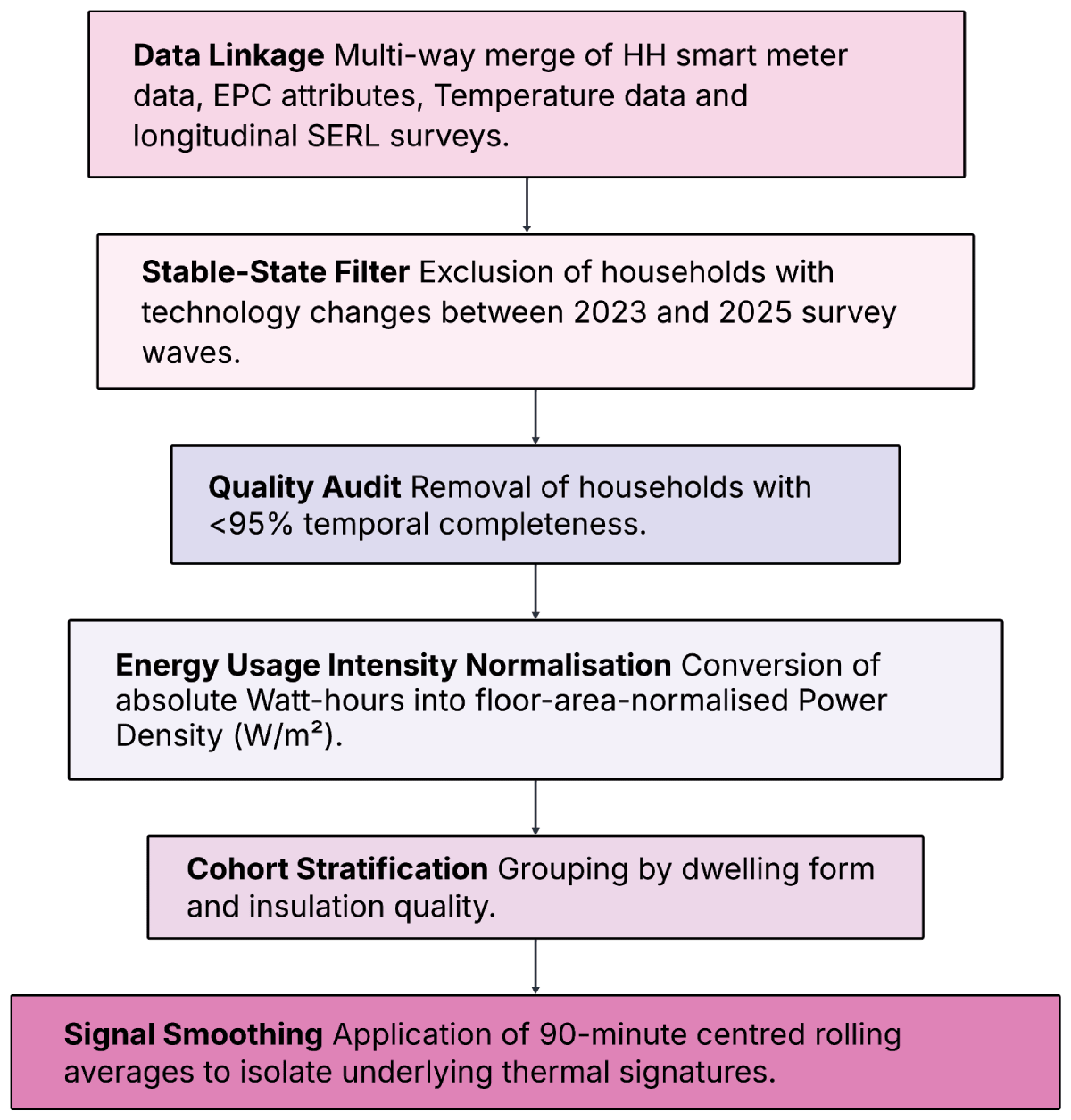
Figure 1
EUI Data Pipeline. Multi-stage processing of SERL Half-Hourly Smart Meter and EPC data to normalise demand (W/m2) and isolate settled technology-fabric groups through stable-ownership filtering.
3 Data
3.1 Data integration and longitudinal consistency
The dataset is derived from the Smart Energy Research Lab (SERL) Observatory (Webborn et al., 2021). To ensure the most robust data linkage possible, we combine:
Half-hourly electricity smart meter data (January 2024–March 2025).
SERL survey data (2023 & 2025): Used to verify technology ownership and occupant demographics at two distinct time points.
EPC Data: Used to extract Total Floor Area (m2) and building fabric attributes.
3.2 Quality control and inclusion criteria
3.2.1 Data completeness and EPC linkage
A primary requirement for inclusion was the successful linkage between smart meter time-series data, the Energy Performance Certificate (EPC) database, and both waves of the SERL Observatory participant surveys (2023 and 2025). Only households with a valid Total Floor Area measurement from the EPC were retained.
The pre-filtering dataset comprised approximately 11,000 households; the post-filtering sample is 1,813. The three main sources of attrition were: (1) failure to match EPC records (~40% of attrition): many SERL households do not have a recent EPC lodged, as EPCs are only required at point of sale or rental; (2) insufficient temporal data completeness (see 3.2.2); and (3) technology changes between survey waves invalidating the stable-ownership criterion (see 3.3). The retained 1,813 households represent a high-completeness, technologically stable subset. The filtering does not introduce systematic bias by building type or tenure, as verified by comparison against the full SERL sample demographics.
3.2.2 Meter reliability and physical plausibility
Smart meter readings quality was ensured by:
Temporal Availability: Only households with ≥95% half-hourly data completeness were included. This threshold was set to ensure that averaged peak demand profiles are not skewed by missing data during key winter peak periods. A household missing 5% of winter half-hours could appear artificially low in weather below 5.5°C.
Plausibility Caps: Any half-hourly interval exceeding 15 kW or 500 W/m2 was flagged and removed as likely meter malfunction. The 15 kW ceiling corresponds to the maximum physical delivery capacity of a standard UK 100 A domestic service fuse, making any sustained reading above this implausible for a single dwelling.
Clock Synchronisation: Intervals with incorrect UTC time-stamps were removed. Without this step, misaligned timestamps would place meter readings in the wrong half-hour slot, causing the 17:00–21:00 peak window to be misrepresented across the cohort.
3.3 Technological stability and settled behaviour
A “Stable-Ownership” filter was applied: households that adopted an HP, installed PV/Battery, or purchased an EV between the 2023 and 2025 surveys were excluded. This ensures the dataset reflects “settled” usage. Without this filter, households mid-transition, still learning a new system or in the first months of HP use, would introduce transient behavioural noise that obscures the underlying long-run energy signature of each technology group.
3.4 Group classification
Households were assigned to mutually exclusive groups (Table 1) based on:
Form: Detached, Semi-Detached, Terraced.
Fabric (Insulation): ‘High-Insulation’ (Cavity or Solid wall insulation present AND loft insulation >200 mm) vs. ‘Low-Insulation’ (uninsulated walls AND loft insulation <200 mm or absent). The term ‘Low-Insulation’ is used consistently throughout.
Table 1
Household stratification and inclusion criteria.
| DIMENSION | CATEGORY | DATA SOURCE | INCLUSION CRITERIA/LOGIC |
|---|---|---|---|
| Physical Form | House Type | EPC | Segmented by: Detached, Semi-Detached, Terraced |
| Building Fabric | High-Insulation | EPC | Walls: Cavity or Solid wall insulation present. & Loft: Insulation thickness >200 mm. |
| Low-Insulation | EPC | Walls: Uninsulated. Loft: Insulation thickness <200 mm or “None.” | |
| Stability | Longitudinal | SERL Survey | Technology status (EV/HP/PV/Batt) must be identical in both 2023 and 2025 survey responses. |
3.5 Climate effect
To ensure a rigorous comparison, results are segmented by Heating Degree Days (HDD) using a base temperature of 15.5°C. The ‘Cold Band’ represents periods where the mean external temperature fell below 5.5°C (high HDD). Note: the 5.5°C Cold Band threshold and the 15.5°C HDD base temperature serve different purposes. The 15.5°C base is a standard UK HDD convention for calculating cumulative thermal demand over time. The 5.5°C Cold Band threshold identifies discrete day-types where instantaneous HP heating demand peaks; it was selected to isolate the highest-stress conditions for distribution network infrastructure. This identifies the peak W/m2 required when thermal lift (the temperature differential the heat pump must overcome between the outdoor air and the indoor heat delivery system, which increases compressor workload and electrical draw) is greatest, and building fabric is under maximum stress, preventing seasonal variations from masking the impact of insulation.
3.6 Establishing the gas-heated baseline
A gas-heated control group was established to provide a baseline for traditional heating demand across different building types. This allows for a comparison between the “As-Operated” profiles of gas-heated homes and those with electrified heating. By observing these two groups, the analysis can identify divergence in peak demand patterns, providing a benchmark to discuss how fabric efficiency might influence domestic energy use in a non-electrified context.
3.7 Structural divergence and confounding variables
This section establishes a baseline using the gas-heated no LCT control group to isolate how physical scale and fabric influence traditional heating demand before comparing these profiles to electrified households. A critical observation in the stratification of this baseline is the structural divergence between building fabric and dwelling scale. Non-Insulated dwellings in the sample exhibit a mean floor area of 82.6 m2, whereas dwellings with improved fabric (Solid + Loft and Cavity + Loft) average 103.7 m2 and 104.4 m2, respectively. This 21% disparity in floor area represents a primary confounding variable. Smaller dwellings inherently possess a higher surface-to-floor-area ratio (greater external envelope exposure relative to internal floor space) and, under standard thermal modelling (assuming uniform occupancy and constant heating setpoints), would be expected to exhibit the highest Gas Power Density (W/m2). However, the 2024–2025 weekday data reveals what could be considered a counterintuitive relationship:
The Cavity Only group reached a peak intensity of 33.85 W/m2, exceeding the 30.66 W/m2 recorded for Non-Insulated homes.
Normalisation Requirement: This data infers that peak power density is not solely a function of insulation status. The normalisation framework (Section 2.1) is therefore essential to isolate energy outcomes from physical scale.
The data indicate that the most thermally inefficient dwellings, on average, demonstrate lower-than-predicted intensity signatures during peak periods. Conversely, dwellings with partial insulation (Cavity Only) demonstrate higher intensity than those with no insulation. By utilising the 2024–2025 peak time weekday window, this baseline captures the current established consumption profiles, providing a control group for comparison against the electrified treatment groups.
These four categories are collapsed into the binary High-Insulation/Low-Insulation split used from Section 4 onward: Solid + Loft and Cavity + Loft as High-Insulation, Non-Insulated and Cavity Only as Low-Insulation.
3.8 Group exclusion and sample attrition
Groups with a sample size of N < 9 were excluded from the primary analysis. This threshold was set because groups smaller than 9 households would produce 95% confidence intervals so wide as to preclude any meaningful comparison with the control baseline. The excluded groups primarily represented uncommon technology combinations (e.g. HP + EV + PV + Battery) where current UK adoption rates remain too low to generate sufficient SERL sample density. These are the configurations most likely to grow in prevalence as the transition matures, making them a priority for future data collection.
3.9 POST-FILTERING cohort sizes
Table 2 lists the cohort sizes after filtering.
Table 2
Cohort Sizes.
| BUILT FORM | TECHNOLOGY GROUP | INSULATION | N | % TOTAL | NOTE |
|---|---|---|---|---|---|
| Detached/Semi | A: PV only +Batt | High-Insul | 45 | 2.5% | |
| Detached/Semi | A: PV only +Batt | Low-Insul | 17 | 0.9% | |
| Detached/Semi | A: PV only | High-Insul | 102 | 5.6% | |
| Detached/Semi | A: PV only | Low-Insul | 30 | 1.7% | |
| Detached/Semi | B: EV only | High-Insul | 29 | 1.6% | |
| Detached/Semi | B: EV only | Low-Insul | 9 | 0.5% | * small sample |
| Detached/Semi | C: HP only | High-Insul | 10 | 0.6% | * small sample |
| Detached/Semi | D: EV + PV + Batt | High-Insul | 21 | 1.2% | * small sample |
| Detached/Semi | D: EV + PV | High-Insul | 10 | 0.6% | * small sample |
| Detached/Semi | E: HP + PV + Batt | High-Insul | 11 | 0.6% | * small sample |
| Detached/Semi | E: HP + PV | High-Insul | 10 | 0.6% | * small sample |
| Detached/Semi | H: Control | High-Insul | 513 | 28.3% | |
| Detached/Semi | H: Control | Low-Insul | 228 | 12.6% | |
| Terraced | A: PV only + Batt | High-Insul | 14 | 0.8% | |
| Terraced | A: PV only + Batt | Low-Insul | 9 | 0.5% | * small sample |
| Terraced | A: PV only | High-Insul | 24 | 1.3% | * small sample |
| Terraced | A: PV only | Low-Insul | 9 | 0.5% | * small sample |
| Terraced | H: Control | High-Insul | 380 | 21.0% | |
| Terraced | H: Control | Low-Insul | 328 | 18.1% | |
| TOTAL | 1,813 | 100% |
[i] * Some have small samples (n = 10–24); findings should be treated as indicative rather than definitive. Group F (HP + EV + PV) Removed due to sample size.
4 Results
4.1 Overview of peak demand and structural divergence
Addressing the research question, how does LCT adoption affect peak electrical power density? The results indicate a fundamental shift in energy demand associated with the transition from traditional gas-led baselines to electrified technology stacks. While Figure 2 shows an 18:00 snapshot that provides a ‘Cold Band’ maximum, the high-intensity windows visualised in Figure 3, in the form of heatmaps, reveal how demand persists across the 17:00–21:00 peak period. When normalised by floor area (W/m2), peak evening electrical demand is increased in homes with HP integration when compared with control homes, whereas EV ownership seemingly shows an increased nocturnal load, with a distinct temporal decoupling from the evening peak.
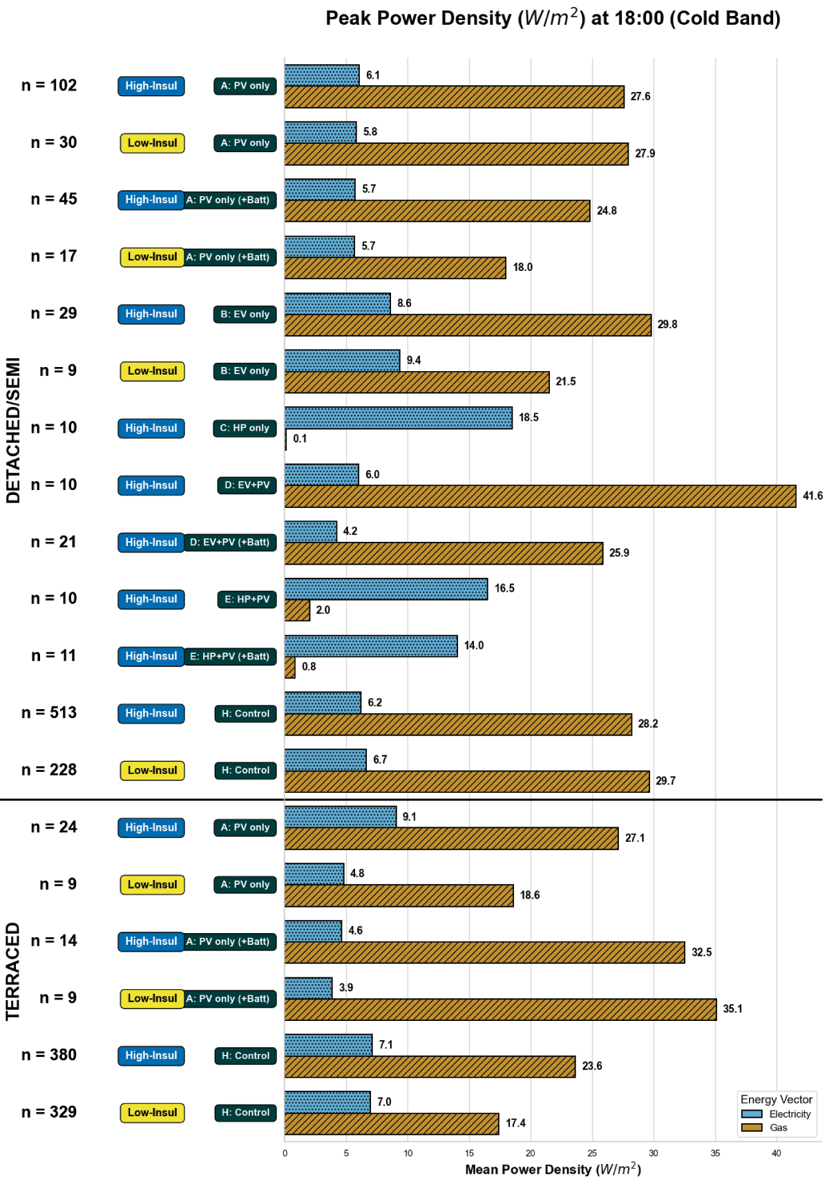
Figure 2
Mean Peak Power Density (W/m2) at 18:00 during Cold Band conditions (<5.5°C). Each group is shown with two bars: blue with dots = electrical intensity (W/m2); hatched orange = gas intensity (W/m2). The bottom bar cluster in each housing-type section represents the gas-heated control group (Group H: no LCTs), providing the baseline against which all technology groups are compared. Top section = Detached/Semi-Detached; Bottom section = Terraced.
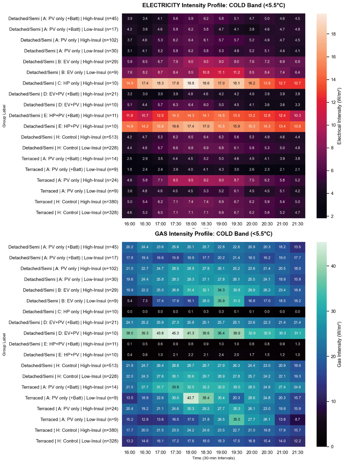
Figure 3
Heatmap of Mean Electrical and Gas Intensity (W/m2) across Technology groups during the 16:00–21:30 Window (Cold Band <5.5°C).
4.1.1 Key observations from peak intensity profiles
Linking back to the research question, does insulation mitigate peak intensification? The heatmap (Figure 3) for the Cold Band confirms that HP demand (Groups C and E) is not merely an instantaneous peak but a sustained high-intensity block. For Group C (HP only, n = 10*, High-Insulation Detached/Semi), electrical demand remains above 17.0 W/m2 for the entire window from 17:00 to 19:30. This suggests that during cold bands, the grid must support a “plateau” of demand rather than a transient spike, significantly increasing the cumulative energy required from local substations.
The electrical intensity profiles for EV-owning households (Group B: EV only, n = 29, High-Insulation, Detached/Semi) show a high degree of variance, with demand jumping from 5.9 W/m2 at 16:00 to 9.4 W/m2 by 18:30. However, the heatmaps illustrate that this remains well below homes with HP (Group C: HP only, n = 10*, High-Insulation, Detached/Semi) levels. The successful shift of charging to the nocturnal window, where demand rises to 8.7 W/m2 at 02:00, could demonstrate the efficacy of ToU tariffs in preventing a further increase during the evening heating window.
The gas intensity heatmap highlights a stark divergence in the Terraced cohort, the bottom third of the heatmap. Group A (PV + Battery) High-Insulation homes maintain a sustained gas intensity above 30 W/m2 between 17:00 and 19:30. In contrast, the Low-Insulation Control (Group H) peaks at only 18.05 W/m2. This indicates that the high-insulation configurations in this sample are drawing higher instantaneous gas loads during peak cold hours than their lower-insulation counterparts, regardless of the underlying cause.
As shown in the electricity heatmap, the homes with the addition of a battery (Group D vs Group B) use less electricity during peak hours. In the Detached/Semi cohort, the battery-equipped EV group (Group D: EV + PV + Battery, n = 21*, High-Insulation, Detached/Semi) maintains a demand of only 4.2 W/m2 at 18:00, compared to 8.6 W/m2 for the EV-only group. The low electrical profile suggests a “peak shaving” effect, where the battery could be absorbing the heavy spikes from EV charging and appliances to give the grid a reduction in peak times.
4.2 The control group: LCT-free homes
This section directly answers: what is the electrical and gas peak demand baseline that LCTs must be measured against? Group H (gas-heated, no LCTs) provides this baseline.
To evaluate the impact of the low-carbon transition, the existing gas-heated building stock (Group H) serves as the benchmark. During cold periods (<5.5°C), these control groups represent the traditional energy profile that electrified technologies aim to displace.
As illustrated in Figure 4, the Detached/Semi-Detached control group exhibits a synchronised peak gas intensity of around 29 W/m2 at 18:00–18:30. This represents the peak coincident demand of the current network. The corresponding electrical load remains considerably lower (approximately 6.2–6.6 W/m2).
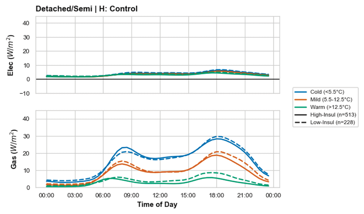
Figure 4
Diurnal Power Density (W/m2) for Group H (gas-heated, no LCTs, Detached and Semi-Detached) during Cold Band (<5.5°C). This is the control baseline against which all technology groups are compared.
Figure 5 displays the equivalent profile for the Terraced cohort, which operates at a lower absolute intensity, peaking at 23.63 W/m2 (High-Insulation) and 17.42 W/m2 (Low-Insulation). The 31.7% higher peak in the “High-Insulation” terraced sample suggests that the baseline for these homes could be influenced by construction typologies (such as solid wall versus cavity masonry), varied occupancy behaviours and internal temperature set-points rather than just the nominal insulation thickness or EPC rating.
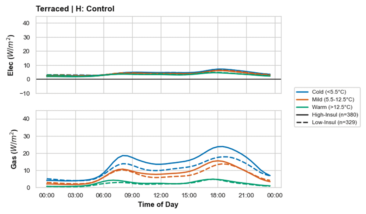
Figure 5
Diurnal Power Density (W/m2) for Group H (gas-heated, no LCTs, Terraced) during Cold Band (<5.5°C).
The diurnal profiles in both figures reveal a rapid ramp-up starting at 16:00. In Detached homes (Figure 4), gas demand nearly triples between 04:00 (3.55 W/m2) and 08:00 (23.05 W/m2). This morning peak and the sustained 18:00 gas peak define the current delivery characteristics of the gas network, boilers and how they are used. While heat pumps typically operate with flatter, elongated profiles because lower peak heating power is typically installed, a result of the high capital cost of the plant per kW compared to gas boilers, this gas peak represents the incumbent thermal demand that must be managed. The challenge for the electrical grid is not necessarily replicating these 29 W/m2 spikes, but rather accommodating the increased baseload (Love et al., 2017) and preventing “re-synchronised” peaks caused by rapid recovery from night-time setbacks (Bernard et al., 2024).
4.3 Heating homes with heat pumps
SMALL SAMPLE NOTE: Group C (HP only, n = 10) and Group E (HP + PV, n = 10) have small sample sizes. The following findings are indicative rather than definitive. This section addresses: to what extent does HP adoption intensify evening peak electrical demand? The results show HPs are the primary driver of Cold Band peak demand intensification.
Figure 6: In High-Insulation Detached/Semi-Detached homes, HPs alone (Group C) exhibited a mean electrical evening peak of 18.5 W/m2, representing a massive shift compared to the control baseline of 6.2 W/m2 (Figure 4).
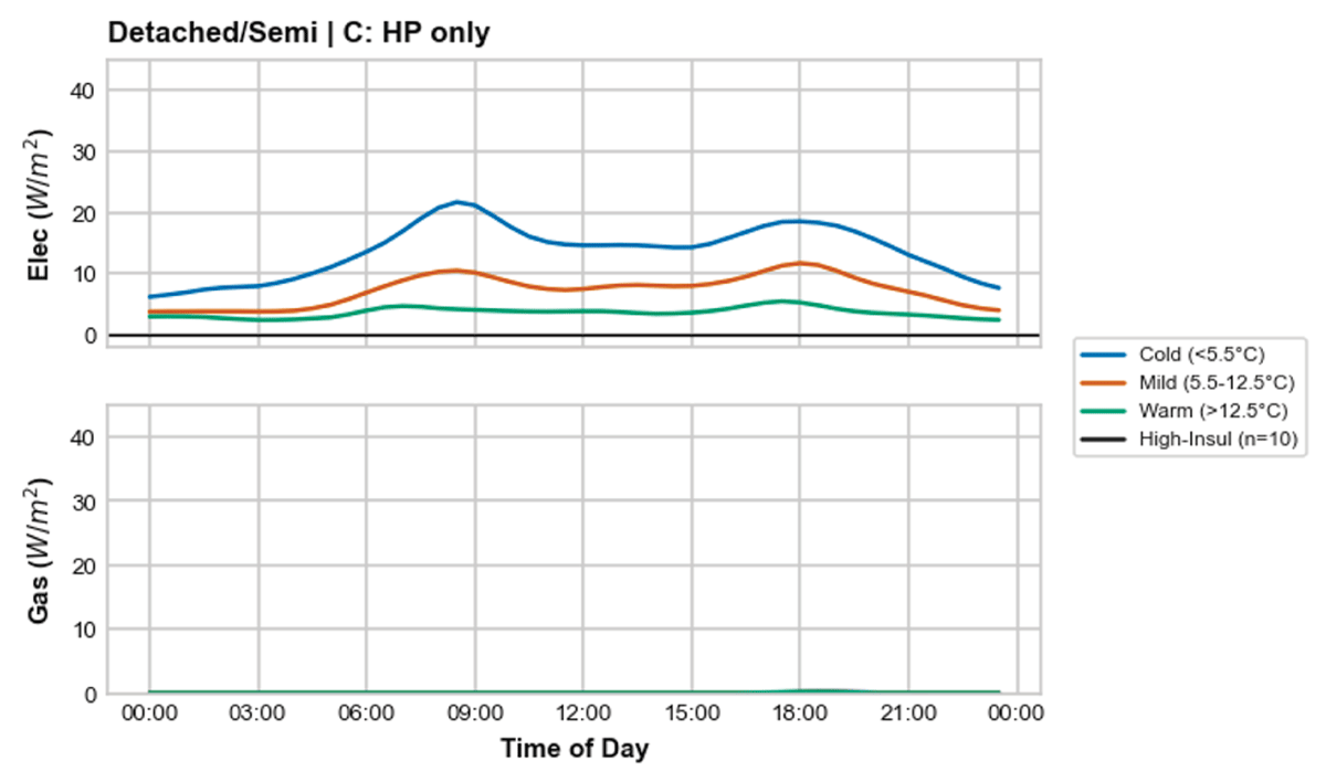
Figure 6
Diurnal Power Density (W/m2) for Group C (HP only, High-Insulation, Detached/Semi-Detached, n = 10*) during Cold Band (<5.5°C). Near-zero gas signature reflects hybrid heating arrangements (gas hob retention or legacy boiler use), not complete fuel displacement.
Figure 7: When local generation is added (Group E: HP + PV), the evening peak remains high at 16 W/m2. Because solar generation is negligible during winter evening peaks, the reduction is minimal.
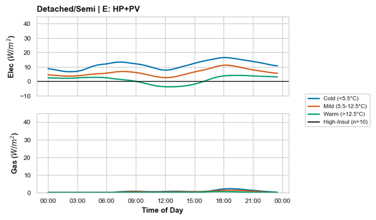
Figure 7
Diurnal Power Density (W/m2) for Group E (HP + PV, High-Insulation, Detached/Semi-Detached, n = 10*) during Cold Band (<5.5°C). Residual gas spikes of 0.82–2.24 W/m2 at 18:00 indicate a hybrid heating reality or oven/stove.
Despite the transition to electrical primary heating, a non-zero gas signature remains evident in the HP cohorts. As observed by Hollick et al. (2026), gas use often persists in heat pump-equipped homes due to the retention of gas hobs for cooking or the use of legacy boilers for peak thermal support. This is reflected in the Cold Band data, where Group E (HP + PV) still exhibits residual gas spikes of 0.82–2.24 W/m2 during the 18:00 window, suggesting that “electrification” in the current housing stock is often a hybrid reality rather than a total fuel displacement.
4.4 Transport: EV integration and battery buffering
This section addresses: does EV adoption intensify the evening electrical peak? The data suggests effective temporal decoupling, likely driven by ToU tariff uptake, consistent with the literature (Bernard et al., 2024; Burger and Rosenow, 2025).
SMALL SAMPLE NOTE: Group D (EV + PV, n = 10) has a small sample size. Findings are indicative.
The EV owning homes data seems to reveal a high degree of ToU tariff uptake, where the potential for a secondary electrical peak is mitigated by off-peak shifting.
As shown in Figure 8, EV-owning households exhibit an evening peak of only 8.62 W/m2 at 18:00 in High insulation homes. The primary charging event is successfully decoupled from the heating peak, shifted instead to the nocturnal window where demand rises to 10.21 W/m2 at 02:00. This reinforces the efficacy of ToU tariffs in protecting the grid during peak evening hours for the charging of EVs.
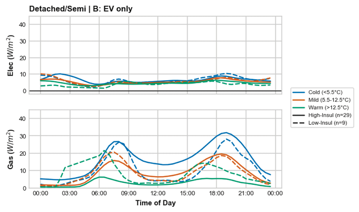
Figure 8
Diurnal Power Density (W/m2) for Group B (EV only, High-Insulation, Detached/Semi-Detached, n = 29) during Cold Band (<5.5°C).
This pattern does not hold uniformly across the fabric strata, however. In Low-Insulation EV-only homes (n = 9), the evening peak is both later and higher, 10.45 W/m2 at 19:00, compared to 8.62 W/m2 at 18:00 in High-Insulation homes, and unlike the High-Insulation cohort, evening demand exceeds the nocturnal charging value (7.02 W/m2 at 02:00) rather than the reverse. Given the small sample size, this should be read as indicative.
Figure 9 illustrates the diurnal profile for households combining EVs with Solar PV. While the 18:00 electrical peak is slightly lower than that of Group B (EV Only) at 6.03 W/m2, the most notable observation is the persistence of high gas demand. During the Cold Band, Group D (EV + PV) records a peak gas intensity of 41.59 W/m2 at 18:00.
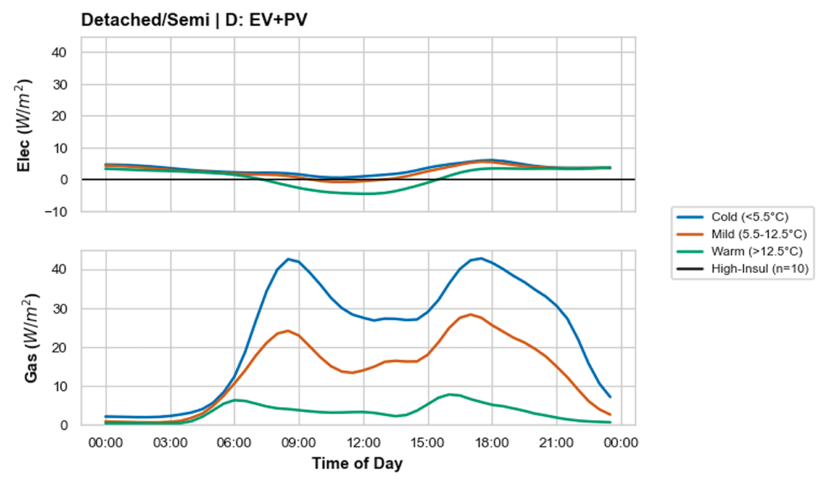
Figure 9
Diurnal Power Density (W/m2) for Group D (EV + PV, High-Insulation, Detached/Semi-Detached, n = 10*) during Cold Band (<5.5°C). High gas demand (41.59 W/m2 at 18:00) confirms a gas-heated home; EV and PV in combination decouple transport load only.
4.5 Solar PV
This section addresses: does PV and battery storage mitigate evening peak intensification? The results show that winter solar yields are insufficient to mitigate evening peaks directly, but battery storage delivers meaningful peak-shaving.
The integration of Solar PV, with and without domestic storage, demonstrates the first stage of relieving pressure on the grid. While winter solar yields are minimal during the evening peak, this data shows the homes containing batteries have a much reduced peak during these colder days.
Figure 10 (Detached/Semi, PV Only): Households maintain an evening electrical peak of 6.05 W/m2 at 18:00; since solar generation has ceased, the PV array provides little mitigation for the evening peak, leaving these homes as heavily dependent on gas as the control group (27.60 W/m2).
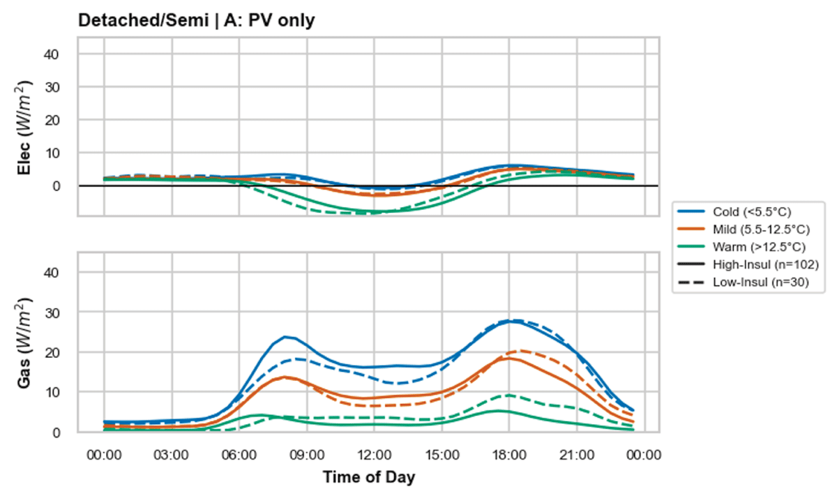
Figure 10
Diurnal Power Density (W/m2) for Group A (PV only, Detached/Semi-Detached) during Cold Band. PV provides no evening peak mitigation in winter; gas heating dominant.
Figure 11 (Detached/Semi, PV + Battery): The 18:00 electrical peak is slightly reduced to 5.72 W/m2, but the profile reveals a significant nocturnal shift; in Low-Insulation homes, electrical demand spikes to 9.20 W/m2 at 04:00, which may indicate a deliberate use of off-peak grid power to prime storage for the following day.
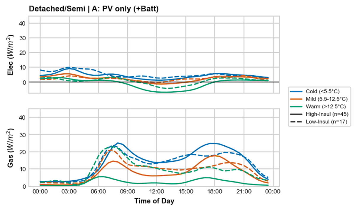
Figure 11
Diurnal Power Density (W/m2) for Group A (PV + Battery, Detached/Semi-Detached) during Cold Band.
Figure 12 (Terraced, PV Only): Standalone solar homes exhibit a sharp evening electrical peak of 9.06 W/m2; this demand mirrors the Control Home consumption, while gas intensity remains high at 27.14 W/m2.
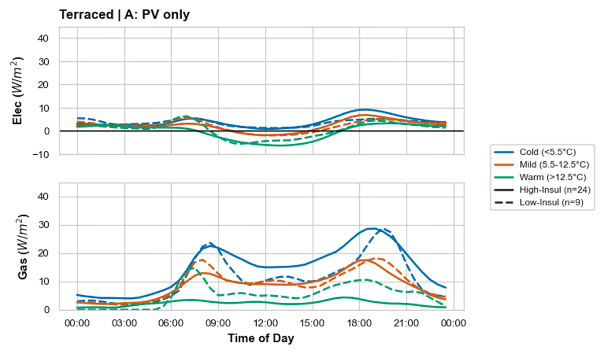
Figure 12
Diurnal Power Density (W/m2) for Group A (PV only, Terraced) during Cold Band.
Figure 13 (Terraced, PV + Battery): The electrical peak is nearly halved to 4.62 W/m2; the electrical usage remains very low, despite a massive, sustained gas peak of 32.55 W/m2.
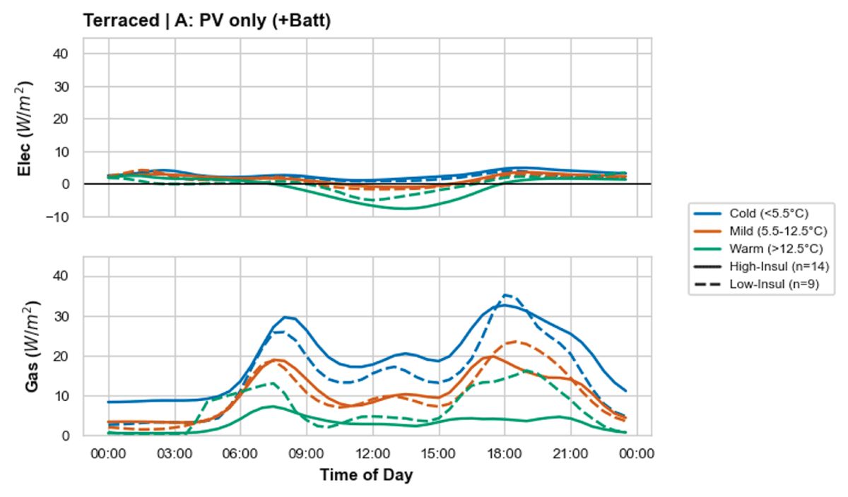
Figure 13
Diurnal Power Density (W/m2) for Group A (PV + Battery, Terraced) during Cold Band.
4.6 Cumulative technology stacking
This section addresses the research question’s final component: does full technology stacking deliver meaningful peak mitigation? The results show a clear reduction in electrical peak demand but highlight that gas heating persistence fundamentally limits whole-home decarbonisation.
The potential for full-home decarbonisation lies in technology stacking, such as the integration of generation (PV), storage (Battery), and demand-side electrification (HPs or EVs). While a comprehensive analysis of the “all-electric” cohort (Group G) was originally planned, the sample size (N) proved insufficient for statistically-significant results and was excluded to maintain the integrity of this study. Instead, focusing on the available integrated cohorts reveals how different separate LCT loads (HP and EV) interact with the use of on-site battery storage and PV.
Figure 14: Integrated Heat Pump, Solar PV and battery (Group E): This cohort represents the vanguard of thermal decarbonisation. In the Cold Band (<5.5°C), these homes effectively reduce their reliance on gas, with demand plummeting to a negligible 0.82 W/m2 at 18:00. The electrical demand profile, peaking at 14.04 W/m2, indicates a managed, stable transition.
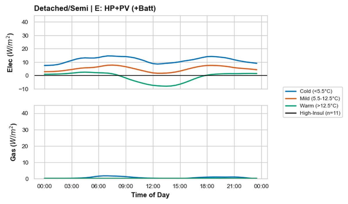
Figure 14
Diurnal Electrical Power Density (W/m2) for Group E (HP + PV + Battery, High-Insulation, Detached/Semi-Detached, n = 11*) during Cold Band. Near-zero gas signature reflects hybrid heating (gas hob retention), not complete fuel displacement.
Figure 15: Electric Vehicle, Solar PV and battery (Group D): While the electrical load is exceptionally low, peaking at just 4.21 W/m2 at 18:00, the thermal profile reveals that the home is still heavily tethered to the gas network, with a peak demand of 25.86 W/m2. This home could be considered storage-rich but demand-poor. Because the home lacks an electrified heating vector (HP), the battery has no “work” to do during the most critical thermal window. This identifies Group D as “Stranded Capacity”: they possess the expensive storage infrastructure, which could help in flattening the grid’s future heating curve, depending on the size of this storage, yet that capacity is currently locked out of the LCT heating transition by a fossil-fuel boiler.
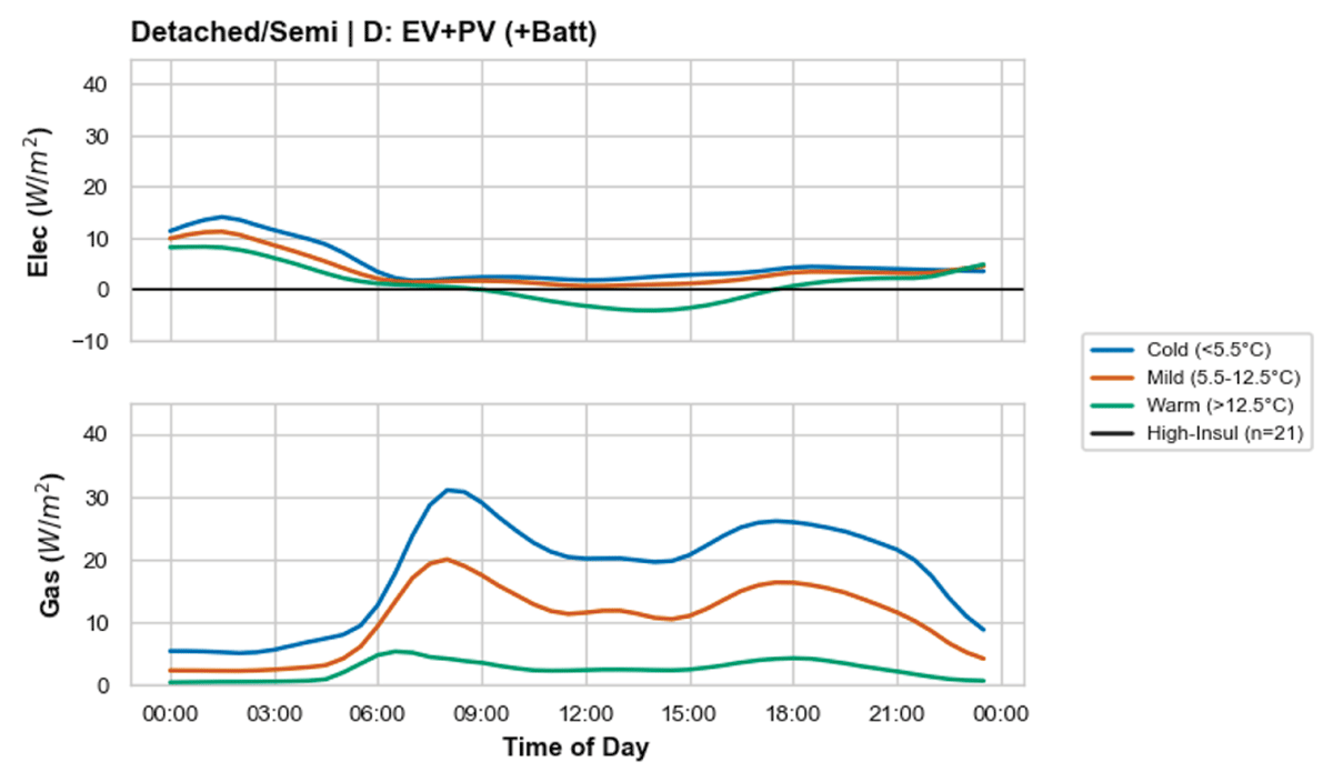
Figure 15
Diurnal Electrical Power Density (W/m2) for Group D (EV + PV + Battery, High-Insulation, Detached/Semi-Detached, n = 21*) during Cold Band. Gas peak of 25.86 W/m2 confirms likely gas-heated home; low electrical figure reflects transport decoupling only.
5 Discussion
This research highlights that while the electrification of heat and transport creates a quantifiable intensification of peak grid demand, the resulting power density signatures are not purely a product of building physics. Instead, they represent a complex interface between fabric performance, mechanical system constraints, and occupant agency. Interpreting these diurnal profiles presents a significant “attribution challenge.” The data allows for the observation of energy outcomes, but without including secondary metadata, specifically occupant intent and financial incentives, defining the specific drivers of these signatures remains speculative.
5.1 The attribution challenge: disentangling physics from behaviour
A core tension in residential energy analysis is the difficulty of isolating the “human” factor from the “technical” factor using 30-minute interval data. While a shift in demand is observed when moving on to electrified heating (Group C), it is impossible to definitively categorise this as “behavioural elasticity” or “mechanical inelasticity” based solely on load profiles.
An observed reduction in energy use in “leakier” homes (the inverse correlation discussed in Section 4.4) could be interpreted as a behavioural response to cost (self-rationing), but it could equally result from differing occupancy patterns or secondary heating usage that is not captured by primary meters. Without longitudinal occupant surveys to verify thermal comfort or set-point preferences, the “Comfort-Taking” and “Self-Rationing” hypotheses remain plausible but unproven drivers of the observed variance.
5.2 The scale disparity: gas vs electricity
The data for Group H establishes a baseline Power Density that underscores the scale of the transition. In the Cold Band, Detached households exhibit a mean gas intensity peak of 28.1 W/m2 (High Insulation). Even when compared to the integrated heat pump stack (Group E: HP + PV + Battery) at 14.1 W/m2, the disparity in magnitude is roughly twofold.
This disparity does not necessarily imply a failure of the building fabric, but rather highlights the different energy delivery characteristics of the two vectors. Gas systems are sized for rapid, high-intensity energy delivery to meet demand “shocks,” whereas electrical systems, particularly HPs, rely on lower-intensity, steady-state delivery. The discussion must therefore focus not on whether the grid can “replicate” the gas peak, but on how the building’s thermal mass can be utilised to move away from high-intensity peaks entirely.
5.3 Implications for distribution network planning and the performance gap
This study adds to the growing body of evidence that EPC-based models systematically misrepresent the “as-operated” behaviour of the GB housing stock. The results provide further empirical weight against the reliability of EPC ratings as a planning tool for grid infrastructure. Where EPC models predict high gas demand in low-efficiency homes, the metered data shows suppressed demand, consistent with the self-rationing behaviour documented by Zapata-Webborn et al. (2024). Conversely, where EPC models might predict lower peak demand in insulated homes, comfort-taking behaviour can produce elevated signatures. This extends the dwelling-level findings of Few et al. (2023) into the context of electrified technology stacks.
Given the scale disparity established in Section 5.2, the implication for network planning is not that the grid must replicate the gas peak, but that pre-heating strategies, where buildings are warmed during off-peak periods and the thermal mass of the fabric retains that heat through the evening, offer a viable pathway to flattening the demand curve. Among heat pump owners, ToU tariff uptake appears relatively high, with Bernard et al. (2024) demonstrating that smart pricing signals can halve evening peak demand without compromising thermal comfort even on the coldest days. The challenge is that this approach remains unavailable to the majority of households still on flat-rate tariffs, and it is this broader population that will need to transition over the coming decade.
A critical and often underappreciated complication for network planners is that gas demand cannot be translated directly into equivalent electrical demand at the point of peak. Three factors make this translation non-trivial. First, the timing of peak demand changes: a gas boiler fires rapidly in response to a thermostat call and delivers high-intensity heat in short bursts, whereas a heat pump operates more continuously across the cold evening hours. Empirical evidence confirms this pattern; Watson et al. (2023) observed that in monitored UK HP households, space heating was drawn almost continuously throughout the evening period, producing a sustained power plateau rather than the sharp, short peak characteristic of gas boiler cycling. This continuous operation is fundamental to HP design: lower-temperature heat delivery requires longer run times to meet the same heat demand. Second, the Coefficient of Performance (CoP) of a heat pump is not constant: under the most challenging cold-weather conditions, precisely the Cold Band periods studied here, CoP declines as the temperature differential between the heat source and delivery system increases. A system with a CoP of 3.5 in mild weather may operate closer to 2.0–2.5 at sub-zero external temperatures (Millar et al., 2025; Hollick et al., 2026), meaning the electrical draw per unit of heat delivered is substantially higher during winter peaks than annual averages would suggest. Third, where a gas boiler can deliver heat at 60–80°C and quickly compensate for a setback period, a heat pump heating to 35–45°C flow temperature cannot recover as rapidly, requiring longer pre-heating windows to achieve thermal comfort, which, if not managed through smart controls, can create re-synchronised peaks as occupants override setbacks on cold evenings (Bernard et al., 2024). Together, these three factors mean that electrical peaks from HP adoption will be more sustained, more sensitive to outdoor temperature, and more structurally embedded in evening demand patterns than a direct substitution of gas demand would suggest. Network planners must therefore account for this temporal reshaping, not simply a scaling of existing peak magnitudes.
6 Limitations
A critical limitation in this analysis is the lack of information regarding ToU Tariffs. The signature observed during the peak window could often be interpreted as a failure to utilise thermal mass for pre-heating.
However, without using the specific tariff structures for these households, it is impossible to determine if this spike is a “behavioural choice” or a “rational economic response.” If an occupant is on a flat-rate tariff, there is no financial incentive to pre-heat; conversely, if they are on a dynamic tariff, the observed peak might represent a mechanical failure of a Demand Side Response (DSR) system rather than a lack of occupant interest. Consequently, the absence of a “shifted load” profile in the data cannot be attributed to a lack of “smart” capability in the building fabric without first accounting for the economic signals being sent to the meter.
A primary constraint of this study is the lack of “whole-dwelling” heat metering. Smart meter data captures primary energy inputs (Gas and Electricity) but does not account for unmetered secondary thermal inputs, such as solid fuels (wood-burning stoves) or portable decentralised electric heaters. Consequently, it is impossible to determine whether a lower-than-predicted primary energy intensity reflects inherent building efficiency or a shift to uncaptured energy vectors. This creates attribution uncertainty in the baseline energy-density signatures.
While the “Best Study” groups (Groups F and G) demonstrate the technical potential of integrated technology stacks, the lower sample sizes (N) for these specific configurations limit the statistical generalisability of the findings.
The categorisation of building fabric is dependent on the most recent EPC filings. However, energy efficiency measures, such as improved loft insulation or draught-proofing, may be implemented without a formal EPC update. This metadata latency introduces a risk of “fabric misclassification,” where dwellings with physically improved thermal performance remain analysed within lower-efficiency brackets, potentially skewing the mean Energy Use Intensity (EUI) calculations.
This study quantifies energy intensity at the individual dwelling level (W/m2). However, this does not account for the “Coincidence Factor” (the probability that multiple dwellings on the same feeder will simultaneously draw peak demand) or local grid topography. The impact of a “Thermal Cliff” is physically determined by the capacity of local distribution infrastructure (e.g., specific LV transformers). While individual dwelling intensity may be quantified, the cumulative risk of “clustering”, where multiple high-intensity cohorts are located on the same feeder, falls outside the scope of this dwelling-level analysis.
7 Conclusions
The data indicate that the UK’s transition toward residential electrification involves a reconfiguration of peak demand profiles that fabric efficiency alone does not fully mitigate. While insulation remains a critical factor in reducing base-load, the high-intensity evening peaks associated with heat pumps and EV charging suggest that “system stacking”, the integrated deployment of HPs, PV, and Battery Storage, could help provide a more robust pathway for managing localised grid stress. The data indicates that the “thermal-behavioural” signature of a home is often more influential than its EPC rating. The study found instances where lower-efficiency homes utilised less energy than their high-performance counterparts. Energy signatures are heavily influenced by varied occupancy behaviours, internal temperature set-points, and specific structural construction typologies that traditional insulation metrics may overlook.
The integrated technology stacks in Group E exhibited a peak electrical intensity of 14.2 W/m2, which, when compared to the 18.5 W/m2 seen in standalone Heat Pumps (Group C) during “Cold Band” weather, represents a 23.4% reduction in peak evening demand. Furthermore, the integration of system stacking achieved a 22% reduction in cumulative evening grid reliance during extreme cold weather (<5.5°C). These integrated systems effectively serve as a technical buffer, absorbing and shifting demand that would otherwise be directed to the distribution network during the critical 18:00 peak.
Regarding transport, the integration of batteries with electric vehicle (EV) charging (Group D) resulted in a 51.2% reduction in grid impact compared to standalone EV charging (Group B: 8.62 W/m2). It is noteworthy that EV loads are already shifting off-peak, likely driven by early-adopter awareness and the automated scheduling capabilities of smart chargers. While the current landscape is still transitioning, with only a small minority of consumers currently utilising ToU or dynamic tariffs, there is a clear upward trend in the adoption of these flexible structures. As it stands, the observed demand spikes often represent a rational economic response to the flat-rate pricing that remains the standard for the majority of the building stock, rather than a fundamental lack of technical flexibility. However, as the market matures over the next 5 to 10 years, the increasing availability and awareness of these ‘smart’ tariffs will be the primary driver in shifting household energy signatures from static consumption to active, price-responsive demand.
As LCTs achieve mass-market penetration, the “thermal shock” signatures observed in this study, characterised by synchronised evening spikes, can be alleviated somewhat through automated, price-responsive demand side response. The future grid will depend not only on how much energy is saved through fabric improvements but on the widespread adoption of system stacking to ensure that the electrification of heat and transport remains within the physical limits of local distribution infrastructure.
7.1 Future research directions
A significant limitation of cross-sectional studies is the substantial heterogeneity across occupants/dwellings. Our future research will prioritise longitudinal monitoring of specific dwellings as they undergo technology upgrades (e.g., the transition from a gas boiler to a heat pump). By tracking the same dwelling and occupant over multiple years, we can isolate the impact of the technology change while controlling for the “human factor.” This will provide empirical clarity on whether the “thermal-behavioural” signature shifts immediately or evolves as the occupant learns the new system.
We will aim to correlate smart meter data with specific ToU or dynamic tariff structures. This will allow researchers to determine if the observed “thermal shock” signatures represent a lack of technical coordination or a rational economic response to flat-rate pricing. Quantifying the relationship between price signals and demand shifting is essential for defining the true “behavioural elasticity” of the building stock.
In the future, rather than relying solely on traditional physical classifications (e.g., “Terraced” or “Semi-Detached”), future research will utilise unsupervised machine learning techniques, such as K-medoids and hierarchical clustering, to identify “energy groups.” This approach would group households based on a broad range of social and physical characteristics. This clustering approach will reveal the actual functional diversity of the housing stock, identifying cohorts of ‘flexible’ versus ‘inflexible’ consumers based on their empirical grid impact rather than on their built form alone.
Data Accessibility Statement
The analysis uses SERL Observatory Data edition 8. The data products accessed were: (1) half-hourly electricity and gas smart meter time-series data; (2) linked EPC records providing floor area and fabric attributes; and (3) SERL participant survey responses from 2023 and 2025 survey waves providing technology ownership verification. The data were provided by the Smart Energy Research Lab (SERL). Due to the sensitive nature of high-resolution smart meter data and re-identification risk, raw data are not openly available. Group-level aggregation and exclusion of cohorts with N < 9 were applied as privacy-protective measures consistent with the SERL data access agreement. Researchers may apply for access via the SERL data access application process at https://serl.ac.uk.
Ethics and Consent
The data used in this research were provided by the Smart Energy Research Lab (SERL). Informed consent was obtained from all participants as part of the SERL Observatory recruitment process. All data accessed was pseudonymised at source; the authors worked only with de-identified data under the SERL data governance framework. Results are reported at the group level only, and cohorts with fewer than 9 households (N < 9) (Webborn et al., 2021) were excluded from all published outputs as a privacy-protective measure to mitigate re-identification risk from high-resolution energy consumption data. Use of SERL survey data from 2023 and 2025 is covered under the same ethical approval framework.