Reduced Order Models for Liquid Hydrogen Pooling and Vaporization Supported by Experiments

1 Introduction

Hydrogen is only a liquid at very low temperatures (approximately 20 K at 1 atmosphere), and if it spills onto a surface, it rapidly absorbs heat from its surroundings, vaporizes and disperses in the atmosphere. Understanding and modeling this type of release is important; to safely utilize this fuel, it is essential to understand where flammable regions occur so that ignition sources can be kept outside of these zones.

Thyer (2003) reviewed data on cryogenic liquid spills, noting only a single study with hydrogen (Takeno et al., 1994). Both the review and the study with hydrogen concluded that the boiling rate of liquid natural gas and hydrogen can often be correlated using a simple 1D heat-transfer conduction model with a boiling rate proportional to t^–1/2 (Thyer, 2003; Takeno et al., 1994). Friedrich et al. (2023) performed vaporization experiments on different substrates and similarly found a t^-1/2 boiling rate for liquid hydrogen spilled onto a solid surface. These studies had some confinement of the hydrogen in a vessel or with walls and did not examine the formation of a pool spreading on an unconfined surface.

Experiments by Royle and Willoughby (2014) observed an approximately 2.14 m long, 1.3 m wide pool for a downward release of liquid hydrogen onto concrete at 60 lpm from a 100 mm height in a 4 m/s cross-wind. The experiments were performed outdoors, so there was variability in the wind speed and direction. Some measurements of concentration demonstrated high variability, with occasional concentrations above 10 vol-% being observed 7.5 m downwind. Hansen and Hansen (2022) summarize experiments performed by the Norweigian Public Roads Administration (Aaneby et al., 2021). In outdoor tests, with 740 and 830 g/s releases downwards from 0.32 m height and wind speeds of approximately 4 and 2.5 m/s wind, temperatures below –200°C were observed at distances less than 0.5 m from the release point, and Hansen and Hansen (2022) claim little evidence of a pool, but Aaneby et al. (2021) describe a pool limited to 0.5 to 1 m from the release point. Indoor tests formed a pool 0.5–1 m from the release point with 500 g/s hydrogen spilling downwards onto the floor with very limited ventilation. In all cases, once the release stops, all remaining liquid quickly vaporizes. Although there have been a handful of other liquid hydrogen spill/release experiments (e.g., Arthur D. Little, Inc. (1960); Witcofski and Chirivella (1984); Schmidtchen et al. (1994); Verfondern and Dienhart (2007); Coldrick (2020); Buttner et al. (2021)), the data on liquid hydrogen spilling onto solid, unconfined surfaces, forming a pool, and dispersing into a cross-wind is quite limited.

Two common modeling approaches for pool formation and vaporization are solving the shallow water equations (Brandeis and Kansa, 1983; Brandeis and Ermak, 1983; Verfondern and Dienhart, 2007), or a simpler force balance driven by gravity (similar to the gas accumulation over spreading pools (GASP) approach of Webber (2012) and the model described by Nguyen et al. (2020)). Both of these approaches will result in a pool size over time, which is a function of the release rate and the heat transfer from the surface to the liquid being spilled, most often solved by assuming that solid surfaces can be treated as a semi-infinite (in depth).

Once the pool size and vaporization rate have been established, these details can be used as a source term for a dispersion model. Dispersion modeling can be accomplished using computational fluid dynamics or using simpler reduced-order models for dispersion. The Hydrogen Plus Other Alternative Fuels Risk Assessment Models (HyRAM+) (Ehrhart et al., 2024) toolkit has a plume dispersion model, but the current publicly released version does not have a model for wind effects, which are very important for these low momentum releases from a large pool. Wind will affect both the momentum and entrainment into the plume.

Experiential measurements of liquid hydrogen pooling and dispersion under well-controlled conditions have been made, and these are compared to newly developed reduced-order models in this work.

2 Approach

3 Results and Discussion

The substrates in the experiments were small for some of the tests and liquid hydrogen could be observed spilling off of them, for high flow rates of liquid hydrogen. For comparisons to the extent of the pool, a test with a low flow rate of hydrogen was used. Example test results with a low hydrogen flow rate are shown in Figure 1. The green dashed vertical lines in Figure 1(a) show the time that the liquid hydrogen began to flow, just after 15:40. The gray shaded region shows the near steady-state data that was averaged, approximately 23.5 min. The red dashed vertical lines indicate the time when the liquid hydrogen stopped flowing. The top frame shows the pressure in the tank, which was slightly above atmospheric and decreased slightly as the spill progressed. The second frame shows the two measurements that were converted into a volumetric flow rate, which is plotted in the third frame. Averaging the two measurements results in an approximate flow rate of 12.5 liters/minute (lpm) of hydrogen. The fourth frame down on the left shows the wind speed, which was approximately 1.9 m/s (4.15 mph), and the fifth frame shows the growth of the pool radius.

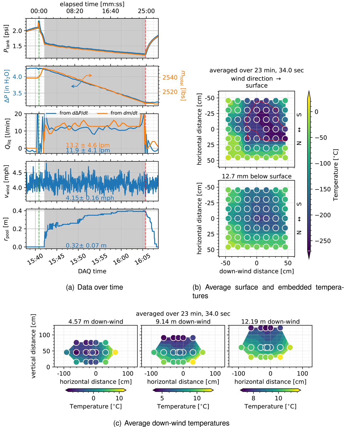
Figure 1

The contour plots in Figure 1(b) are average measurements of the temperatures at the surface (top) and 12.7 mm below the surface (bottom). The pool radius at each point in time was calculated from the instantaneous surface temperature measurements. Any temperatures below 53 K were assumed to be liquid hydrogen, and the area that was covered by liquid hydrogen was converted into a circular radius dimension. The red line shown in the upper plot of Figure 1(b) shows an approximate isocontour at 53 K; the approximate dimensions of the average pool. The pool is not centered on the substrate, but is being blown down-wind slightly and seems to flow in the southern/negative horizontal direction, perhaps due to a slight slope to that side, or an unevenness of the wind.

The three contour plots in Figure 1(c) show the average down-wind thermocouple temperatures at three down-wind locations. Temperatures are lowest towards the middle and top of the measurements, and also increase going downwind (note the different temperature scales for each of the frames). Because the flow rate of hydrogen was so low, the temperatures are fairly close to ambient (at the edges of the plots); in other words, the mole fraction of hydrogen is low.

Figure 2 compares the three different pooling modeling approaches to the data from the experiment of Figure 1. The blue line shows the result of the engineering model described by Eq. 3. The engineering model predicts the largest pool of the three models, and overpredicts the radius in this case. The orange line is the result of the GASP model, described by Eqs. 4 and 5. With the properties used, however, there were issues getting the ODE solver to converge, and the frictional force needed to be increased by a factor of 15 to get the model to integrate. Nonetheless, the radius predicted is very near the experimental results. Finally, the shallow water equations, given in Eqs. 8 and 9, result in a prediction of pool radius that is much smaller than was observed experimentally. Other simulations using these models (not shown) showed similar trends of the engineering model always predicting the largest pool radius, the shallow water equations the smallest, and the GASP model somewhere in-between. The GASP and shallow water equations are both currently slow to solve due primarily to tracking the pool radius over time to determine the annular conductive heat flux. Additional work on the models is needed to increase the speed of solutions, and hopefully improve the range of material properties (e.g., substrate conductivity, substrate thermal diffusivity) for which a solution can be found.

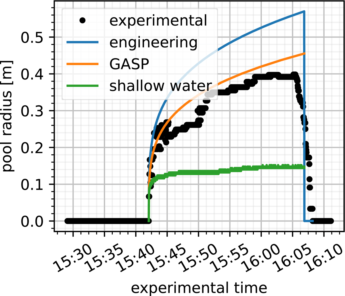
Figure 2

Since there are challenges in predicting the pool radius over time, and previous work showed that CFD models for dispersion were relatively insensitive to the pool radius (Mangala Gitushi et al., 2023), the dispersion model was tested for its sensitivity to pool radius. The left-hand frames of Figure 3 show the 4% mole fraction contour for a 1 m diameter source pool, and the right-hand frames for a 0.5 m diameter source pool for two hydrogen flowrates and 3 wind speeds. A red dashed line on the plot also shows the vector to the tip of the 4% mole fraction contour and the angle of that line is shown in red text. Aside from the bulging contour near the plume origin (x < 0), the contours are nearly identical. The bulge is an artifact of displaying the plume as its trajectory rotates from the vertical release to the nearly horizontal wind-driven dispersion near the pool source, while it is diluted greatly by wind-driven entrainment. In a real release, one would expect the average mole fraction contour to be smooth all the way down to the pool. The larger pool has a barely perceptible longer profile in the x-dimension. A higher flow rate of liquid hydrogen results in a more upward-driven plume (it starts with additional upward momentum), and also results in a longer plume with more flammable mass contained within.

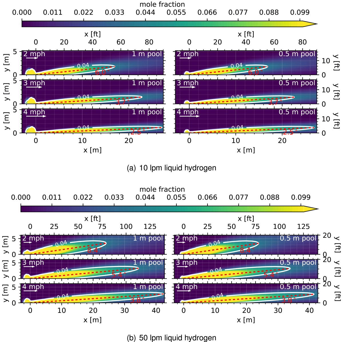
Figure 3

Due to uncertainty with the pool model (and the independence of plume dispersion on the pool radius), the dispersion model was compared to experimental data using an average experimentally measured pool radius as the source of hydrogen. The experimentally measured average mass flow rate and wind speed were also used in the model. The wind was given an upward trajectory of 5° above horizontal because the experimental configuration had a ramp leading up to the substrate that was not directly on the ground. Figure 4 shows the experimental data compared to the HyRAM+ model for two experiments with different release rates of liquid hydrogen of 15 and 45 g/s. Both the data and the model contain upward sloping plumes, and the high mole fractions extend further downwind as the hydrogen release rates increase. However, the mole fractions predicted by the model are much higher than those observed experimentally; there is much more spreading and dilution in reality than is predicted by the model. A more diluted, wider plume is also clear from the side profiles. In particular, Figure 4(a) shows an entire simulated mole fraction field that is less than 0.04 for the slice that is –61 cm from the center. The experimental plume, on the other hand, has mole fractions that are greater than 0.08, at least in the part of the slice that is 4.57 m downwind of the pool. The profiles further show that the average experimental plume is not centered on the axis. Video evidence also showed that the condensed moisture tilted in the negative horizontal direction. Obstructions (such as cameras and data acquisition equipment) upwind of the release are suspected of causing the wind to deviate slightly from the blast tube axis.

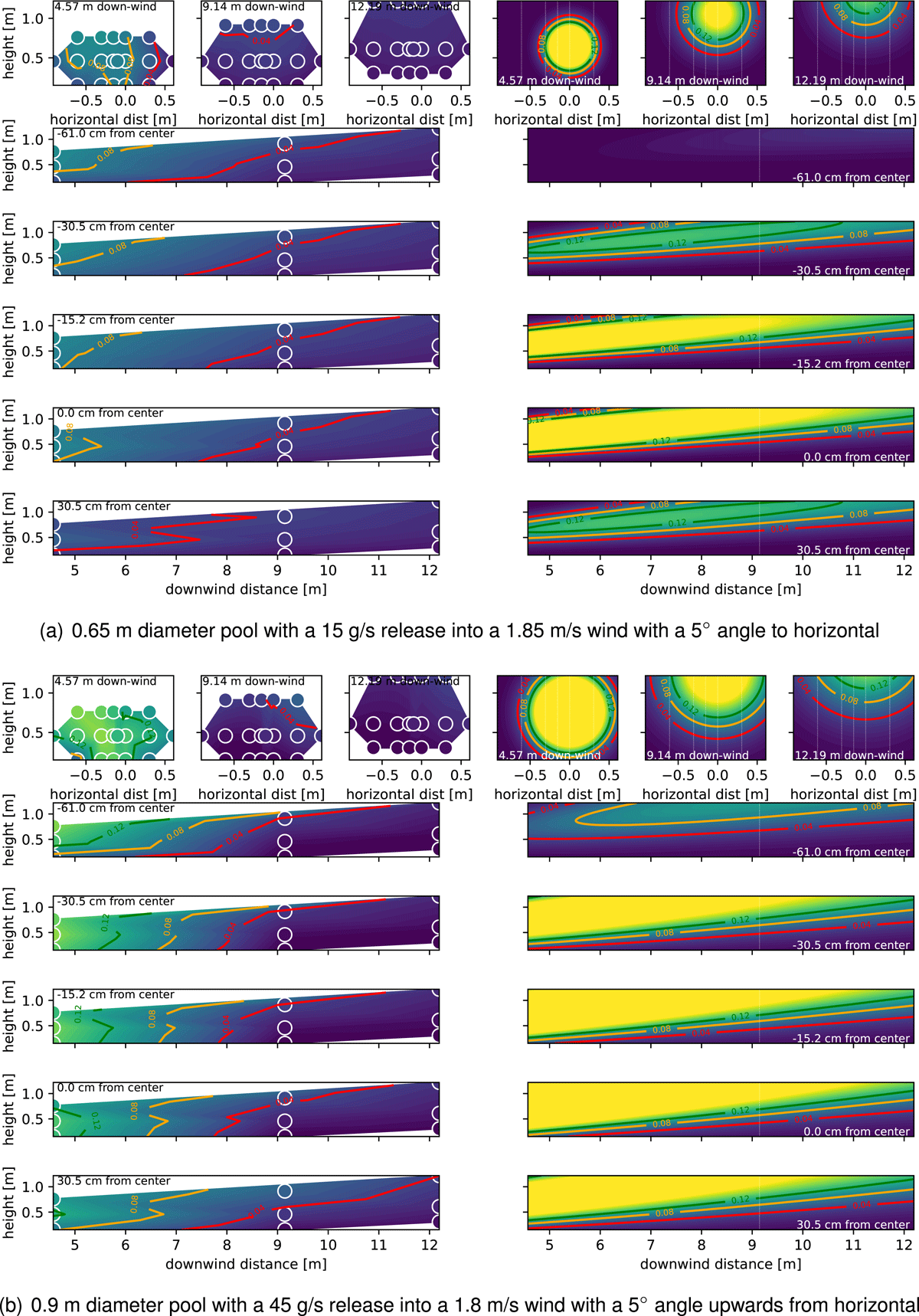
Figure 4

The amount of dilution in the model is easily controlled by the entrainment coefficients, $c_{\parallel }$ and $c_{\perp }$. In Figure 5, both $c_{\parallel }$ and $c_{\perp }$ were varied, to 0.9 and 1.8, respectively. In this case, the extent of the plume and mole fractions are significantly reduced, and the plume is much wider, but the upward trajectory of the plume is also reduced. As the entrainment of air increases (due to the significant increase in $c_{\parallel }$), the buoyancy of the plume decreases, since hydrogen is the buoyant component of the plume, and if there is less hydrogen in the plume, there is commensurately less buoyancy. A thorough comparison and automated minimization of error between the model results and all of the experimental data with additional flow rates of hydrogen, additional cross-wind speeds, and other substrates are needed to see if additional tuning of the entrainment coefficients can improve the agreement between the model and the data.

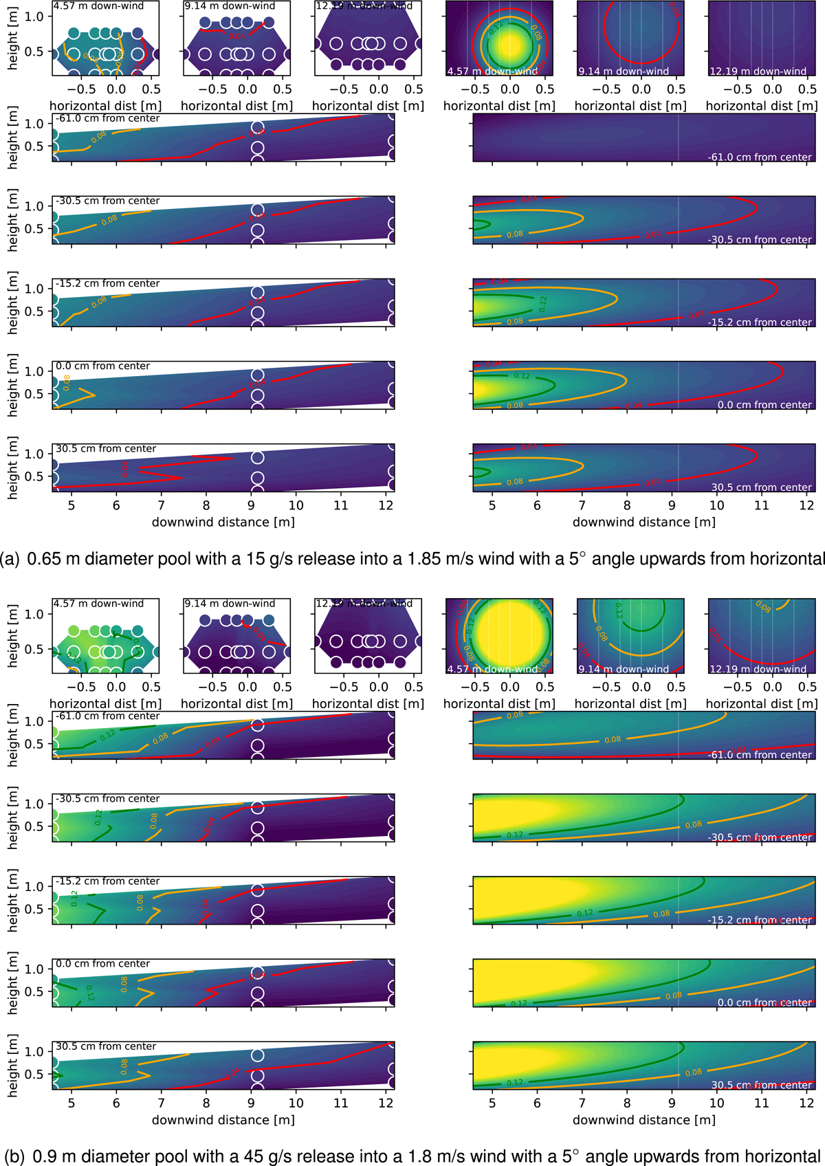
Figure 5

4 Summary and Conclusions

Three different models for pool formation over time are described in this work. An algebraic engineering model overpredicted the pool radius over time; the GASP approach seemed to agree with the experimental data, while a solution of the shallow water equations underpredicted the experimentally observed pool radius. The GASP approach and the shallow water equations have issues with solution stability for certain scenarios and are also slow to solve. Both of these models need additional work to address these deficiencies.

A fast-running dispersion model that is an extension of a plume model in HyRAM+ is also described in this work. The HyRAM+ plume model was modified to include the effects wind has on the momentum of a plume, as well as how wind affects the entrainment of air into the plume. The pool radius is an input to the plume model, and it was demonstrated that the pool radius has little effect on the downwind dispersion of the plume, at least for the limited pool radii (0.5 m versus 1 m) and low winds (< 4 mph) tested in this work. This means that the accuracy of the pool formation is not critical to understanding the dispersion of vaporizing liquid hydrogen spills.

The dispersion model was then exercised, using parameters and data from two different experimental spill rates of liquid hydrogen onto concrete, to assess the accuracy of the model. With the initial empirical coefficients for wind entrainment, the predicted mole fractions were much higher than those observed experimentally. Increasing the parallel driven entrainment coefficient lowered the predicted mole fractions, but also decreased the predicted buoyancy of the simulated plumes. The agreement with the data was improved slightly, but the model needs additional tuning.

In future work, the pooling model will be linked more closely with the dispersion model, and additional optimization of the entrainment coefficients will be made. The optimization will be automated and will use the entire dataset from the pooling experiments that were performed, which includes additional variations in wind speed, spill rate, and substrate beyond what is presented in this work. In addition to the vaporization data presented in this work, literature data will also be used to determine the entrainment coefficients. It is possible that the entrainment coefficients are not simple values but are a function of the experimental parameters, as is the case for momentum and buoyancy-driven entrainment in the HyRAM+ model. This model will be incorporated into the HyRAM+ toolkit and will be useful in assessing the safety of liquid hydrogen systems and the characteristics of specific scenarios that involve spills of liquid hydrogen in an open environment with a cross-wind.

Author Contributions

Ethan Hecht developed and implemented the models, led the experimental campaign, analyzed data, and authored this work.