The DISCHA Engineering Tool for LH2 Tank-to-Tank Transfer Operations

1 Introduction

Enhancement of the safety and efficiency of liquid hydrogen transfer technologies (tank-to-tank) in public areas for mobile applications (trucks, ships, stationary tanks) is the primary goal of the EU-funded ELVHYS project, within the framework of which the current work was performed.

In the present contribution, the DISCHA integral code (see Venetsanos & Giannissi, 2017; Venetsanos, 2018; Venetsanos, 2019; Venetsanos, 2020; Venetsanos, et al., 2021a; Venetsanos, et al., 2021b; Venetsanos, 2021c; Venetsanos, 2024), originally developed for accurate physical properties and discharge calculations, is extended for multizone tank modelling following Machalek, et al. (2021) and Wang, et al. (2022) and is validated for tank self-pressurization against the NASA multipurpose hydrogen test bed (MHTB) tests (Hastings, et al., 2003) and for tank-to-tank LH2 transfer against the NASA non-vent fill experiments (Moran, et al., 1991).

DISCHA calculates accurate single-phase physical properties using Helmholtz free energy-based equations of state for hydrogen and other substances, while it employs the homogeneous (ideal) mixture model (HEM) approach for two-phase conditions. DISCHA has a user-friendly Python-based (tkinter) graphical user interface, connected to Fortran-based dynamic libraries via Ctypes Python library. It can handle a user-defined number of tanks and a user-defined number of transfer (discharge) lines. Each line connects two tanks. A line is made up of a user-defined number of pipes. A pump can also be added to the transfer line by specifying the pump’s characteristic curve. The flow through the transfer lines is modelled using a method that accounts for phase change, friction, area change and heat transfer through the pipe walls. The maximum (choked) flow through the transfer lines is calculated using the Possible Impossible Flow (PIF) algorithm. The tank modelling is outlined in the next section. Heat transfer through the tank walls can be calculated by solving the 1D energy equation inside the wall, taking into account the wall’s physical properties.

2 Modelling

Tank modelling in DISCHA can be performed either with single-zone or with multizone modelling. The tank multizone model used is based on the earlier work of Machalek, et al. (2021) and Wang, et al. (2022). The model considers three zones inside the tank: zone 1 for the liquid part, zone 2 for the vapour part (ullage) and zone 3 for the assumed massless interface in between. All three zones share the same pressure but may have different temperatures. The interface is considered to be always at saturation temperature. The liquid phase may be either saturated or subcooled. The vapour phase may be either saturated or superheated. The basic conservation equations are given below.

Mass conservation (zone 1):

Mass conservation (zone 2):

Volume constraint:

Energy conservation (zone 1):

Energy conservation (zone 2):

Energy conservation (zone 3):

The heat fluxes from zone 2 to the interface (2S) and from the interface to zone 1 (S1) are obtained from the relations below, where the heat transfer coefficients (α’s) are calculated using natural convection Nu correlations for stable stratification over horizontal surfaces, e.g., that of McAdams, or as proposed in Nellis & Klein (2009). Note that stable stratification exists above the horizontal liquid–vapour interface when vapour is superheated and stable stratification also exists below the interface when the liquid is subcooled.

In the equations above, subscripts 1 and 2 represent the liquid and vapour phases, respectively; h denotes the specific enthalpy; u the specific internal energy; ρ the density; V the volume; A the surface (of the liquid–vapour interface or the internal tank wall of zone 1 or zone 2) and ${\stackrel{\cdot }{m}}_{i,\mathit{\text{in}}}$ and ${\stackrel{\cdot }{m}}_{i,\mathit{\text{out}}}$ the mass flow rates in or out of the tank (from zone 1 or zone 2). The K coefficients in equation (7) account for non-equilibrium. Their value was set to 0.1, following Wang, et al. (2022).

The conservation equations of the single-zone tank model can be easily derived by summing the corresponding liquid and vapour equations above.

Mass conservation (whole tank):

Energy conservation (whole tank):

In the case of the single-zone model, equations (8) and (9) are solved using an explicit Euler scheme for the new density and internal energy, respectively, from which the remaining thermodynamic conditions (temperature, pressure, vapour quality, enthalpy, entropy, etc.) can be iteratively derived.

In the case of the multizone model, the algorithm is more complex. An explicit Euler scheme is used that is similar to the single-zone model. The mass transfer rate from zone 1 to zone 2 (evaporation rate) ${\stackrel{\cdot }{m}}_{12}$ is first calculated from equation (6), also using equation (7). Equations (1) and (3) are solved next for the new mass and internal energy of zone 1 (bottom part of the tank) and equations (2) and (4) are solved for the new mass and internal energy of zone 2 (ullage). Then the following iterative procedure is applied over pressure until the zone volumes satisfy equation (3): For each pressure considered, pressure and zone internal energy define the thermodynamic state, i.e., all the other thermodynamic properties, which are iteratively calculated here. From the calculated zone densities and known zone masses, one can obtain the zone volumes and then check whether the convergence criterion is satisfied.

It should be noted that, in the abovementioned iterative procedure over pressure, the liquid phase may appear within the ullage or/and the vapour phase appear within the bottom liquid part of the tank. These may occur, for example, with top spray filling of a tank or two-phase bottom filling conditions. In such situations, the liquid phase, which appeared in the ullage, is instantaneously moved to the bottom part of the tank, and vice versa: the vapour phase which appeared in the bottom part of the tank is instantaneously moved to the ullage.

3 Model Validation

3.1 Tank self-pressurization

3.1.1 Experiments

The tank self-pressurization experiments were performed at the NASA MHTB. The structure of the MHTB tank was simplified as a vertically cylindrical tank with two standard ellipsoidal heads at the bottom and top, similar to Wang, et al. (2022). The tank had a volume of 18.09 m³, a diameter of 3.05 m and a cylindrical height of 1.525 m. The height of each ellipsoidal head was one quarter of the tank’s diameter. The experimental conditions are provided in Table 1.

Table 1

Experimental conditions of the MHTB tank.

TEST #	INITIAL LIQUID FILL (%)	P1 (kPa)	TOTAL HEAT POWER (W)
1	25	122.1	18.8
2	90	113.3	71.3
3	50	122.1	18.7
4	50	111.6	51.8

3.1.2 Simulations

Figure 1 shows a comparison between predicted and experimental ullage pressure time evolution for MHTB tests 1–4. The agreement obtained with the multizone model is reasonably good. The additional simulation of test 4 using the single-zone model shows that single-zone modelling significantly underestimates tank self-pressurization.

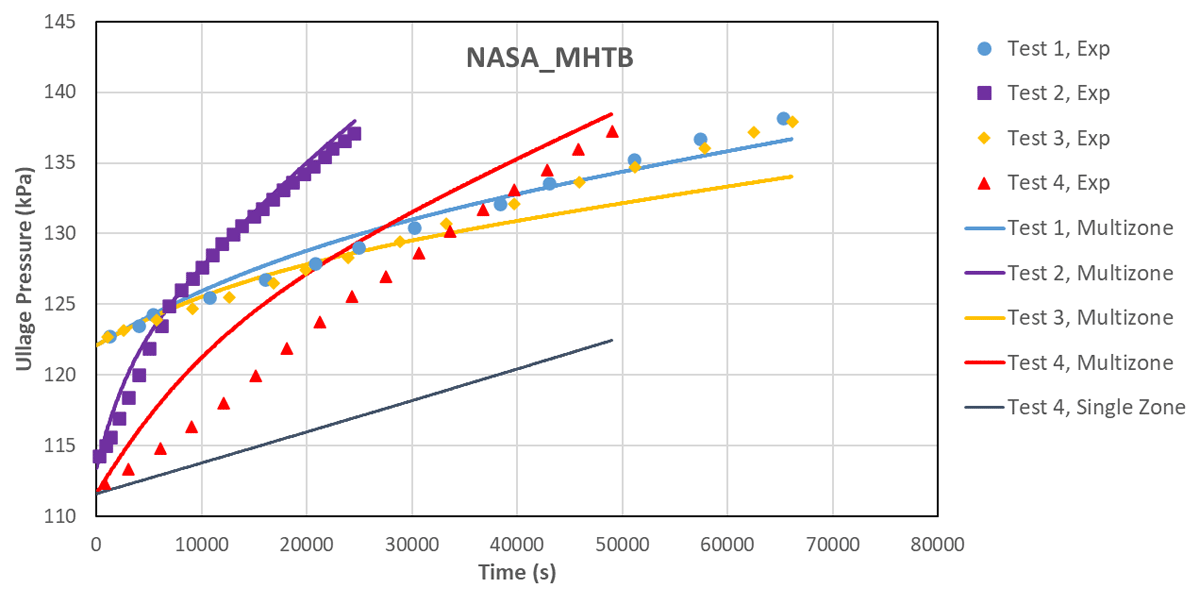
Figure 1

In the simulations, the proportion of heat leaking from the external environment into the ullage was assumed to be half of the heat leaking from the external environment into the liquid. Additionally, a 0.1 K superheat of the vapour phase and subcooling of the liquid phase was assumed. A similar approach was applied in Wang, et al. (2022).

3.2 No-vent tank filling

3.2.1 Experiments

The experiments were performed using the CCL-7 test rig. The rig contains a supply dewar and two interchangeable receiver dewars. The supply dewar is a vacuum-jacketed stainless steel cylindrical tank equipped with multi-layer insulation (MLI) within the vacuum annulus, with an internal height of 54 inches (1.372 m), an inside diameter of 22 inches (0.559 m) and an internal volume of approximately 10.8 cubic feet (306 L).

The receiver dewars are of similar construction to the supply dewar. The small receiver (for which experimental results are reported) has an internal height of 20 inches (0.508 m) and an internal diameter of 12.5 inches (0.3175 m), resulting in an internal volume of 1.2 cubic feet (34 L).

The overall heat flux for all three tanks was experimentally determined, and ranges from 1 to 10 Btu/hr•ft² (3.2–32 W/m²) depending on the fill level and test fluid (nitrogen or hydrogen).

A total of 42 no-vent fills were performed with the small, 34-liter receiver tank: 19 top spray, 7 upward pipe discharge and 16 bottom diffuser tests. Figure 2 illustrates the three fill configurations tested.

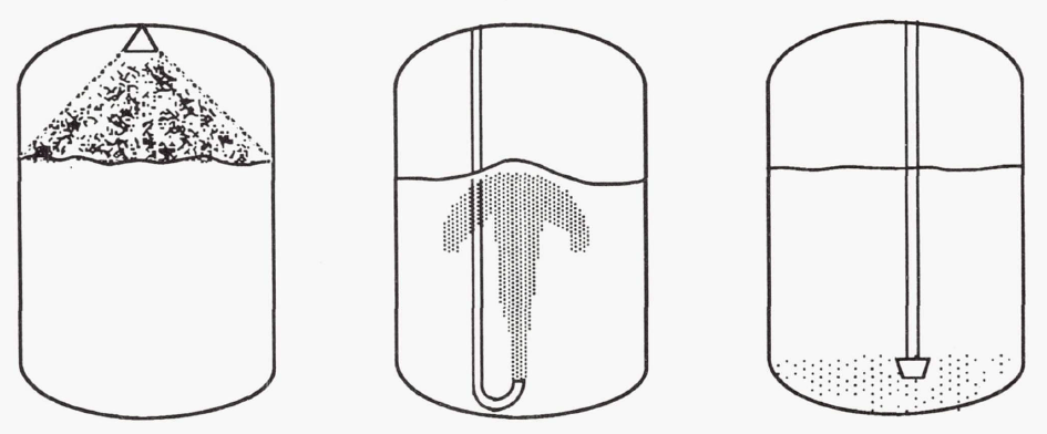
Figure 2

Regarding instrumentation, temperatures were measured with type-T (copper–constantan) thermocouples and silicon diodes, and thermistors were used to indicate the presence of liquid or vapour. Pressure transducers were also used to provide continuous pressure measurement throughout the system. Finally, each tank was equipped with a capacitance-type level probe which was used to calculate the liquid fill level.

3.2.2 Simulations

The DISCHA simulations were performed as follows. Two vertical cylindrical tanks were introduced through the code’s interface, the supply tank and the receiver tank. The supply tank initial conditions were set as per Tables 2 and 3. These correspond to subcooled liquid hydrogen. The supply tank’s initial conditions were assumed to remain constant (in time). The receiver tank was assumed to be initially at the experimentally measured pressure shown in Tables 2 or 3 and at the corresponding saturation temperature with an initial liquid fill level as shown in these tables. All the simulations were performed with a filling line of zero length. The hole’s diameter was tuned to produce approximately the experimentally observed mass flow rate shown in Tables 2 or 3. In the program interface, the filling line was set to connect the bottom of the supply tank with the bottom of the receiver tank for the bottom filling simulations and the bottom of the supply tank with the top of the receiver tank for the top spray simulations. Both tanks were assumed to be thermally isolated from the external environment. Normal hydrogen properties were calculated with the Helmholtz free energy-based equation of state given in Leachman, et al. (2009).

Table 2

Top spray test conditions (1: supply tank, 2: receiver tank).

TEST #	P1 (Pa)	T1 (K)	P2 (Pa)	T2 (K)	MFR (g/s)	INITIAL LIQUID FILL (%)
9093A	206843	17.9	26890	16.6	15.1	4.0
9094A	206843	19.2	26890	16.6	27.2	0.0
9094B	206843	19.3	24132	16.3	22.7	0.0
9094C	206843	19.2	26890	16.6	17.4	0.0

Table 3

Bottom diffuser test conditions (1: supply tank, 2: receiver tank).

TEST #	P1 (Pa)	T1 (K)	P2 (Pa)	T2 (K)	MFR (g/s)	INITIAL LIQUID FILL (%) IN RECEIVER TANK
9088B	206843	19.5	25511	16.5	11.3	4.0
9088C	206843	19.5	20684	16.0	28.7	5.5
9081G	206843	18.5	22753	16.2	31.8	8.0
9088G	206843	18.1	23442	16.3	32.5	7.2

Bottom diffuser filling was used in test 9088B. The experimentally observed mass flow rate was approximately achieved with a pipe diameter of 1.85 mm. The results of the DISCHA simulations for test 9088B are compared to the experimental data in Figure 3. This shows the pressure history and the liquid level as % full by volume for the receiver tank. The figure includes predicted results for a mass flow rate slightly higher than that experimentally reported (for a 2 mm hole diameter). In both cases, the model qualitatively captures the experimentally observed physical behaviour. The quantitative agreement is observed to be better with a slightly higher mass flow rate.

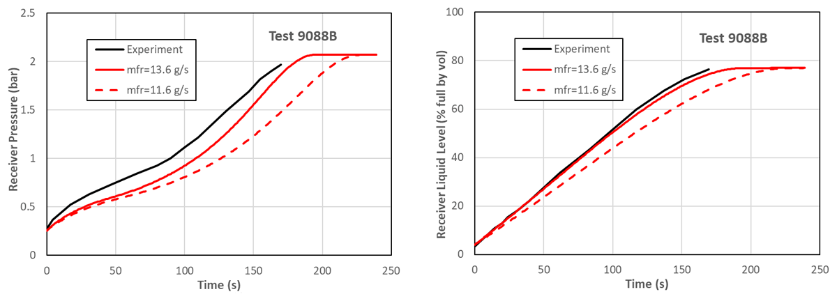
Figure 3

Top spray filling was used in test 9093A. The pipe diameter was tuned (set to 2 mm) to produce approximately the experimentally observed mass flow rate shown in Table 2. The results of the DISCHA simulations for test 9093A are compared to the experimental data in Figure 4. This shows the receiver tank pressure and liquid level histories. The figure includes predicted results for a mass flow rate slightly higher than that experimentally reported (for a 2.2 mm diameter). In both cases, the model qualitatively captures the experimentally observed physical behaviour. Quantitatively, the agreement is shown to be better with a slightly higher mass flow rate.

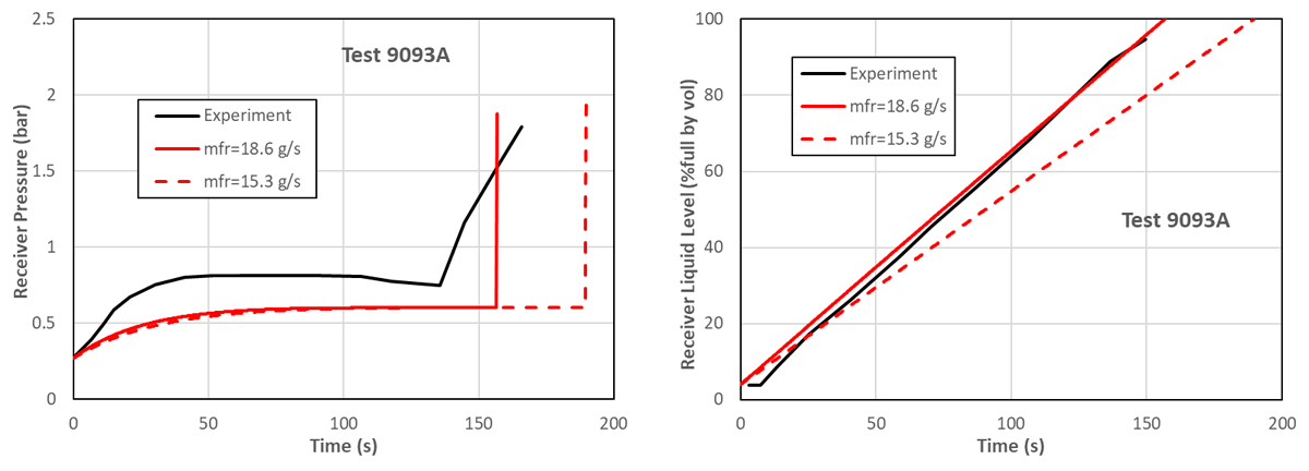
Figure 4

The effect of the inlet liquid temperature on the pressure vs. the fill level response was experimentally investigated and it was found that pressure rises at a lower rate in the receiver tank as the inlet temperature is decreased for all three filling type cases. The DISCHA simulations of tests 9088C, 9081G and 9088G, when compared to the corresponding experimental data in Figure 5, confirm the experimentally observed behaviour/effect.

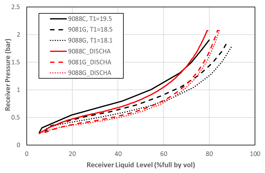
Figure 5

The effect of the inlet liquid mass flow rate on the pressure vs. the fill level response was experimentally investigated and it was found that for higher flowrates, the tank pressure as a function of fill level is reduced. Figure 6 shows predictions for experiments 9094C, 9094B and 9094A (increasing flow rate order) and comparisons with the experimental data. It can be observed that, in the predictions, the above effect is reproduced when comparing tests 9094B and 9094A, but not 9094C and 9094B. This model behaviour and probably also the experimental behaviour might be due to the fact that parameters other than the mass flow rate differed slightly between the considered experiments.

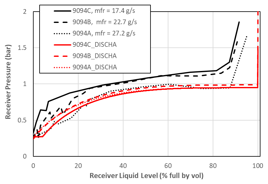
Figure 6

In order to obtain a clearer picture of the effect of the inlet liquid mass flow rate on the pressure vs. the fill level response as predicted by the model, simulations were performed where the only parameter changed was the mass flow rate (by adapting only the hole’s diameter accordingly). Figure 7 shows these simulations with all other conditions remaining exactly the same as for tests 9088B and 9093A, for bottom diffuser and top spray fillings, respectively. It can be observed that the model shows no effect of the inlet liquid mass flow rate on the pressure vs. the fill level response, in contrast to the experiments. Of course, if flow rate is increased, then pressurization occurs more quickly, as shown in Figures 3 and 4.

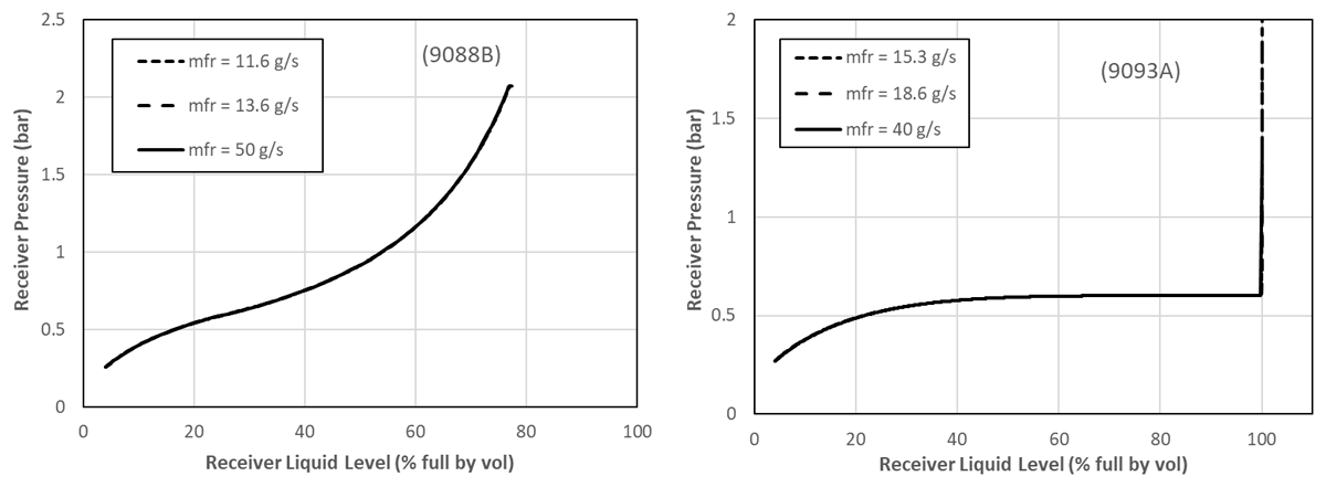
Figure 7

4 Model Application

4.1 No-vent filling of a 400 L tank

We consider the non-vented filling of a LH2 vertical cylindrical tank (receiver) that is 400 L in volume to be representative of the size of the tank of a heavy-duty vehicle. The supply tank is considered to be a 12 m³ vertical cylindrical storage tank, 2 m in diameter. The two tanks are connected with an assumed 30 m long, 2.54 cm diameter transfer line ending in a 10 mm nozzle that is 5 cm in length. The line starts from the bottom of the supply tank and ends at the bottom of the receiver tank, for bottom filling, or at the top of the receiver tank for top filling. The receiving tank is assumed to be initially at 1 atm saturated vapour conditions. The supply tank conditions are either 2 or 5 bars, saturated or subcooled liquid. In the subcooled cases, the supply tank temperature was assumed to be 19 K for both 2 and 5 bars. In the simulations, the multizone model was only applied to the receiver tank. The single-zone model, with pressure kept constant (as an assumption instead of an energy balance), was applied to the supply tank. Keeping the supply tank pressure constant during the transfer could be achieved in practice by extracting liquid from the bottom of the tank, vaporizing it and then redirecting it to the ullage. Also, in the simulations, all components were considered adiabatically isolated (via MLI or other means). Investigating the heat transfer interactions with the external environment was out of the scope of the present work, but it could be considered in the future.

Figure 8 shows the predicted receiver tank liquid level (% full by vol) vs. time. It can be observed that both the initial conditions in the supply tank and the filling method (bottom or top filling) play an important role. With saturated initial conditions in the supply tank, it is not possible to reach 100% full receiver tank conditions; in fact, the filling levels achieved are very low (less than 50%). Filling levels increase if the liquid inside the supply tank is subcooled. Filling levels also increase with pressure in the supply tank. Even with the higher of the two pressures considered (5 bars) and bottom filling, the target tank would not be filled more than approximately 80%. Only with top filling would the 400 L tank be filled up to 100% for both pressures, with subcooled conditions inside the supply tank.

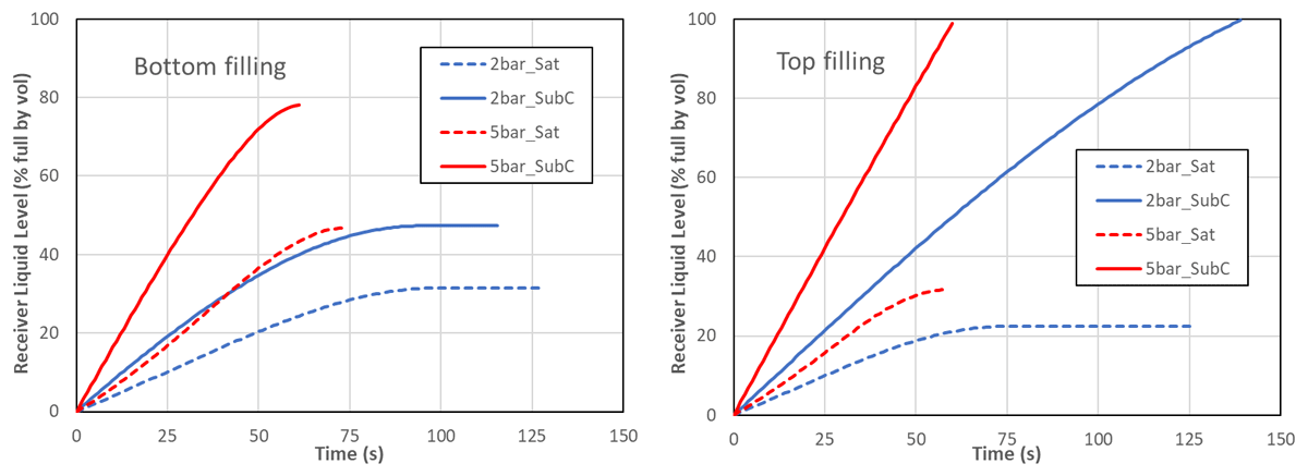
Figure 8

Figure 9 shows the predicted mass flow rates vs. time corresponding to Figure 8. The flow rates are reduced to zero as the filling is almost complete and the pressure in the target tank is approaching that in the supply tank. The pressure responses of the receiver tank are shown in Figure 10.

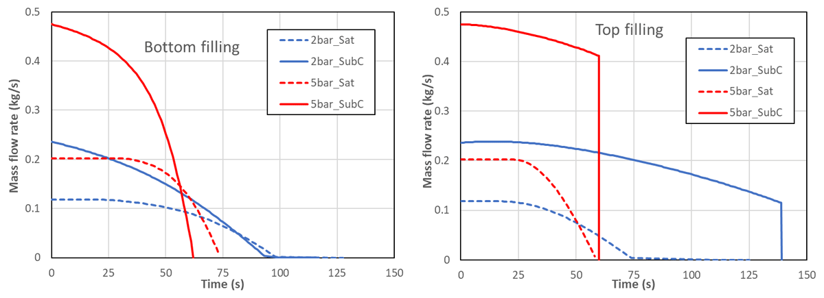
Figure 9

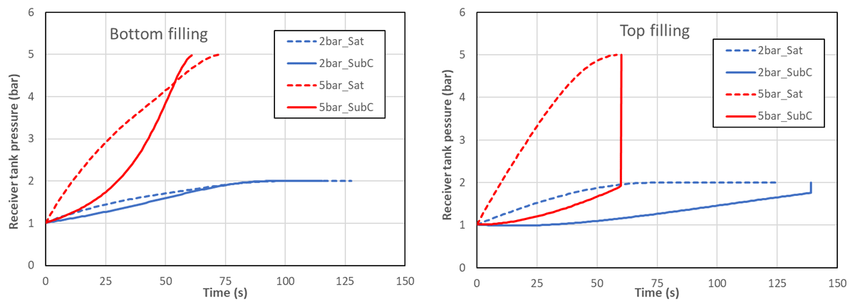
Figure 10

5 Conclusions

The DISCHA integral code was extended for multizone tank modelling. Associated validation was performed for a) tank self-pressurization against the NASA MHTB experiments and b) tank-to-tank LH2 transfer against the NASA non-vent fill experiments.

The code predicted the MHTB tank pressurization history in reasonable agreement with the experimental data for the four experiments considered.

Regarding the NASA non-vent fill experiments, the code reproduced reasonably well the experimentally observed different behaviour of the top spray and bottom diffuser fillings concerning receiver tank pressure and fill level response. Regarding the effect of the inlet liquid temperature on the pressure vs. the fill level response, it was found that pressure rises at a lower rate in the receiver tank as the inlet temperature is decreased in accordance with the experiments. Regarding the effect of inlet liquid mass flow rate on the pressure vs. the fill level response, the present model shows no effect for the conditions examined.

DISCHA was applied to simulate the non-vented filling of a 400 L LH2 tank, a size representative of a heavy-duty vehicle, from a 12 m³ stationary supply tank, through a long transfer line at various supply tank initial conditions and using either bottom or top filling methods. It was shown that a) final filling levels can be very low in certain conditions, b) filling levels increase with pressure and subcooling in the supply tank and c) with subcooled conditions in the supply tank, top filling is more effective than bottom filling and can theoretically achieve 100 % full receiver tanks, while, with saturated conditions in the supply tank, bottom filling is more effective, although the filling levels achieved will remain low.

Disclaimer

Views and opinions expressed are those of the author(s) only and do not necessarily reflect those of the European Union or the Clean Hydrogen Partnership. Neither the European Union nor the Clean Hydrogen Partnership can be held responsible for them.