
1.0 Introduction
Hydrogen is emerging as a versatile carbon free energy carrier, offering a viable pathway to decarbonize applications currently depending on fossil fuels. With its high gravimetric energy density and versatility, liquid hydrogen (LH2) enables zero-emission solutions for aviation, maritime shipping, and heavy-duty vehicles—sectors where electrification remains challenging. The ongoing work within the AppLHy! (Transport and Application of Liquid Hydrogen) project is a key component of the TransHyDE flagship initiative, one of three large-scale hydrogen projects funded by Germany’s Federal Ministry of Education and Research (BMBF) under its National Hydrogen Strategy (Fuhry et al., 2025). AppLHy! focuses on advancing LH2 infrastructure by addressing critical challenges in liquefaction, storage, transportation, and application. It develops technologies such as centrifugal LH2 pumps, hybrid pipelines (combining superconducting power cables with LH2 transport), and LH2-cooled superconducting motors for high-efficiency applications in aviation, heavy transport, and industry. The project also explores supply chain optimization through modeling and pilot programs, aiming to enable scalable, energy-dense LH2 solutions for decarbonizing mobility and energy sectors.
The physics-based model for simulating the LH2 tank is primarily governed by heat transfer mechanisms, which dominate under both normal and abnormal conditions. Key studies (Daigle et al., 2011; Machalek et al., 2021; Osipov et al., 2011; Petitpas, 2018; Ustolin et al., 2023) highlight three critical pathways of heat transfer: the liquid-vapor interface, flash evaporation in liquid and wall-to-fluid interaction. Typically, heat conduction through imperfectly insulated tank walls and convection into the liquid and gas phases govern boil-off within the tank, driving evaporation at the interface. Thermodynamic models couple energy and mass conservation with phase change dynamics, in which interfacial heat flux drives vapor generation. In the event of vacuum insulation failure, convective and radiative heat transfer from the ambient environment to the tank wall intensifies, inducing strong boiling at the wall-liquid interface and significantly increasing boil-off rates. Conversely, a rapid pressure drop (e.g., venting via a burst disc) reduces the saturation temperature, triggering flash evaporation at the liquid-vapor interface. These transient phenomena are modeled through non-equilibrium thermodynamic approaches, capturing the abrupt phase changes. Recent work integrates lumped parameter codes (Daigle et al., 2011; Machalek et al., 2021; Osipov et al., 2011; Petitpas, 2018; Ustolin et al., 2023; Venetsanos et al., 2024 and 2025; Xu et al., 2023) to simulate the coupled effects of heat transfer, phase change, and pressure dynamics, with validation against experimental data. These models are essential for optimizing insulation design, predicting potential hazards, and ensuring the safe storage and transport of LH2.
Computational fluid dynamics (CFD) has proven to be a valuable tool for analyzing the physical phenomena and evaluating the fluid dynamics and heat transfer performance of liquid hydrogen tanks (Cirrone et al., 2023; Kartuzova et al., 2024; Leuva et al., 2012; Wang et al., 2013). Research focused on developing and refining CFD models to enhance understanding of complex processes, including the intricate dynamics of heat and mass transfer during condensation and evaporation. However, these models require validation against experimental data to ensure their reliability in predicting LH2 tank behavior under both operational and accident conditions. Additionally, for long-term transient system simulations, the computational expense of CFD can pose significant challenges. The lumped parameter method offers a solution to the computational time constraints of CFD by simplifying the system dynamics. However, its effectiveness relies on the accuracy of heat transfer models, such as those describing flash evaporation during pressure drops in accident scenarios.
Over an extended period, significant research efforts (Gopalakrishna et al., 1987; Liao, Y. and Lucas, D., 2017; Saury et al., 2002 and 2005) have been dedicated to investigating the phenomenon of flash evaporation in water pools. Gopalakrishna et al. (1987) conducted experiments on water desalination, investigating flash evaporation with various initial liquid temperatures, superheats, salt concentrations, and distilled water heights. By measuring the liquid level using a cathetometer, they developed empirical correlation to determine the mass of water evaporated due to flashing at any given moment. Saury et al. (2002 and 2005) conducted experimental studies to examine the effects of initial water level and depressurization rate on flash evaporation within a flash chamber. Like Gopalakrishna experiments, Saury experiments also involved initial liquid temperatures, superheat levels, and initial water heights. The investigation primarily focused on assessing how initial water height influences key flash evaporation characteristics, including flashing time and the mass of liquid evaporated. The evaporated mass was determined through an energy balance applied to the liquid within the flash chamber. However, prior research indicates a significant gap in understanding the flash evaporation of LH2. Models or empirical correlations derived directly from LH2 flash evaporation experiments are scarce.
This research aims to develop a physics-based model to simulate hazardous scenarios in LH2 systems, so that it provides an accurate temporal source term for CFD simulation involving the AppLHy! project. The study focuses on creating a predictive model for LH2 tanks, namely the whole non-equilibrium model with new flash evaporation correlation and performing comprehensive analyses to assess tank inside behavior and hydrogen gas source release into the atmosphere under different thermal insulation conditions. The LH2 tank model accurately determines heat transfer and blowdown rates under both normal operating conditions (e.g., boil-off) and abnormal scenarios (e.g., vacuum insulation failure). These simulations enable comprehensive risk assessments, supporting the design of safer hydrogen infrastructure by quantifying potential hazards and informing mitigation strategies.
2.0 Methodology and Case Studies
2.1 General modeling framework
The current LH2 tank model operates under a non-equilibrium assumption, meaning the liquid and vapor phases are not thermally equilibrated and therefore require separate mass and energy balance calculations (Daigle et al., 2011; Machalek et al., 2021; Osipov et al., 2011; Petitpas, 2018; Ustolin et al., 2023; Venetsanos et al., 2024 and 2025). These phases are separated by a thin, massless saturated vapor film. Figure 1 illustrates the mass and energy conservation principles for a two-phase cryogenic hydrogen system, where subscripts V and L denote the vapor and liquid phases, respectively. The model incorporates a comprehensive heat transfer framework that accounts for conduction, convection, and boiling under high heat flux conditions.
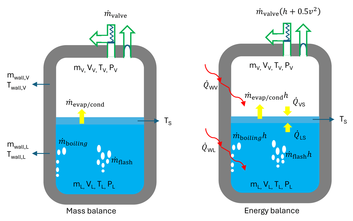
Figure 1
LH2 tank non-equilibrium model.
This non-equilibrium model was developed using components from Sandia’s HyRAM Python framework (Groth and Hecht, 2017), including orifice, notional nozzle, and fluid objects. The modeling in this paper is influenced solely by the orifice flow mode. The flow is choked through the orifice since the ambient pressure is much smaller than the pressure in storage. The thermal conditions at the orifice are solved using an assumed isenthalpic expansion. The notional nozzle model (e.g., Birch model) is applied for external flow calculations, the internal tank dynamics are governed by the orifice discharge. Hydrogen properties are derived from the CoolProp package (Bell et al., 2014), which utilizes a Helmholtz energy-based equation of state. The system simulates compressible flow in networks consisting of pressure vessels, orifices, and valves, represented as interconnected nodes or paths. Specifically, the tank is modeled as a two-node system: one representing the liquid phase and the other the vapor phase. Figure 1 illustrates the mass and energy exchange mechanisms between these nodes.
2.1.1 Governing equations
In the non-equilibrium tank model, the governing equations differ between the liquid phase node and the vapor phase node. The liquid and vapor mass balances are expressed as:
where mL, mV represent the liquid and gas masses, respectively. The evaporation/condensation rate () and boiling rate () are detailed in Sections Liquid-Vapor Interface and Wall-to-Fluids. The condensation rate is calculated using the same formulation as for evaporation, but it is triggered when the vapor temperature exceeds the saturation temperature at the liquid-vapor interface. The resulting mass flux is simply assigned a negative value to indicate mass transfer out of the vapor phase. The energy balances for liquid and vapor phases are given by (Daigle et al., 2011; Osipov et al., 2011):
where uL, uV are the liquid’s and vapor’s internal energy, and represent the heat transfer rate from the liquid and vapor to the film surface, respectively, and hL,sat, hV,sat denote the liquid and vapor phase enthalpy under saturated condition, while hV is the vapor enthalpy and v is the gas velocity through the valve or burst disc. The term pdV accounts for the quasi-static work associated with the compression or expansion of the control volume. Note: The change in mass should be considered in the left-hand term of the energy balance equations.
2.1.2 Liquid-vapor interface
In this model, the thermodynamic state of each phase (superheated, subcooled, or saturated) is determined by its internal energy. The liquid and vapor phases are separated by the massless thin film, which is maintained at the saturation temperature corresponding to the vapor pressure, that is, Ts = f(PV). The evaporation/condensation rate is governed by the heat transfer to the liquid-vapor interface. Applying an energy balance to the thin film yields the evaporation/condensation mass flow rate:
where is the latent heat of vaporization, evaluated at the film temperature Ts. The heat transfer rate between phase α (liquid L or vapor V) and the film occurs through conduction and, in specific scenarios, convection. Conductive heat transfer () is always present, while convective heat transfer () arises only due to natural convection. This occurs in the vapor phase if the vapor is cooler than the film, or in the liquid phase if the liquid is hotter than the film—that is, when a denser fluid overlies a less dense one within the same phase. The total heat transfer is the sum of these contributions:
A boundary layer (BL) model, initially developed by Osipov et al. (2011) and later adapted by Petitpas (2018), accounts for temperature gradients in the liquid and vapor regions. However, simulations using this approach exhibited high sensitivity to BL length parameters. Machalek et al. (2021) proposed an alternative method but did not justify the selection of BL lengths. For simplification, the conductive heat transfer between the film and hydrogen in phase α is modeled using the following correlation (Daigle et al., 2011):
where 𝜅 is the thermal conductivity, Cp and Cv are the heat capacities, 𝜌 is the density, and T is the temperature of the phase α (liquid or vapor). As is the cross-sectional area of the interface, g is the gravitational constant, β is the thermal expansion coefficient, and µ is the dynamic viscosity.
2.1.3 Flash evaporation
The non-equilibrium model of the LH2 tank does not account for liquid superheating accurately when only considering evaporation at the interface. Especially when the superheat is large, the flash could occur. The flash evaporation model assumes the use of the current interface heat and mass transfer framework during sudden pressure drops caused by burst disc opening. Flash evaporation within the liquid occurs when the superheat limit is reached, leading to the formation of vapor bubbles. These bubbles nucleate, rise through the liquid, and subsequently break through the free surface.
Saury et al. (2005) proposed a model of the flash evaporation system by dividing it into two subsystems in thermodynamic equilibrium. The first subsystem consists of a liquid mass, m – dm, at temperature T at time t, which transitions to a liquid mass, m – dm, at temperature T + dT at time t + dt. The second subsystem comprises a liquid mass, dm, at temperature T at time t, alongside a vapor mass, dm, at temperature T + dT at time t + dt. By neglecting thermal losses to the chamber walls and interactions with the surrounding fluid, they derived a heat balance equation to describe the energy dynamics of the flash evaporation process.
By integrating over time , the temporal evolution of the evaporated mass is derived. Given the relatively low temperature range, the thermophysical properties of the liquid, such as density, latent heat of vaporization, and specific heat capacity, are assumed to remain constant throughout the flash evaporation process. Consequently, the following equation is obtained to describe the energy balance and mass transfer dynamics:
By differentiating the derived equation with respect to time and assuming the physical properties of the fluid remain constant, the evaporation mass flow rate is also determined:
The uncertainty in the evaporated mass, calculated using above Equation 11, was analyzed in Saury et al. (2002). The results indicate that the relative uncertainty remains below 12% compared to experimental data. However, the temperature T and gradient are dependent variables, requiring implicit calculation for their solution.
In additional experiments (Gopalakrishna et al., 1987), the temporal evolution of the flashed mass for each experimental run was determined. A least-squares curve-fitting method, utilizing Equation 12, was applied to derive the parameters specific to each run. The experimental data, representing the mass of flashed vapor as a decay function of time, exhibited a strong correlation with the fitted model.
where the time constant , unit 1/s.
Dimensional analysis conducted in Saury et al. (2005) introduced dimensionless numbers for each physical quantity. Correlations were established to describe the evolution of the dimensionless initial mass flow rate, , as a function of other significant dimensionless parameters, including the superheat , depressurization rate vp, and the initial liquid height H. Specifically, a new correlation, Equation 15, was proposed linking the dimensionless maximum flash mass flow rate, , to the dimensionless superheat Jacob number Ja, the dimensionless depressurization rate vp,dem, and the dimensionless initial water height Hdem.
where the dimensionless numbers are .
As this study was conducted using distilled water (Saury et al., 2005), the range of validity for the proposed correlations remains an open question. Comparisons between the predicted and experimental values of the dimensionless initial mass flow rate, , and the flash mass flow rate, , are presented in Figures 2 and 3. These comparisons indicate that the biases are generally small, with good overall agreement between predictions and experimental data. However, at a low depressurization rate of vp = 0.67 bar/s, a relatively larger deviation is observed at the onset of the flash evaporation process.
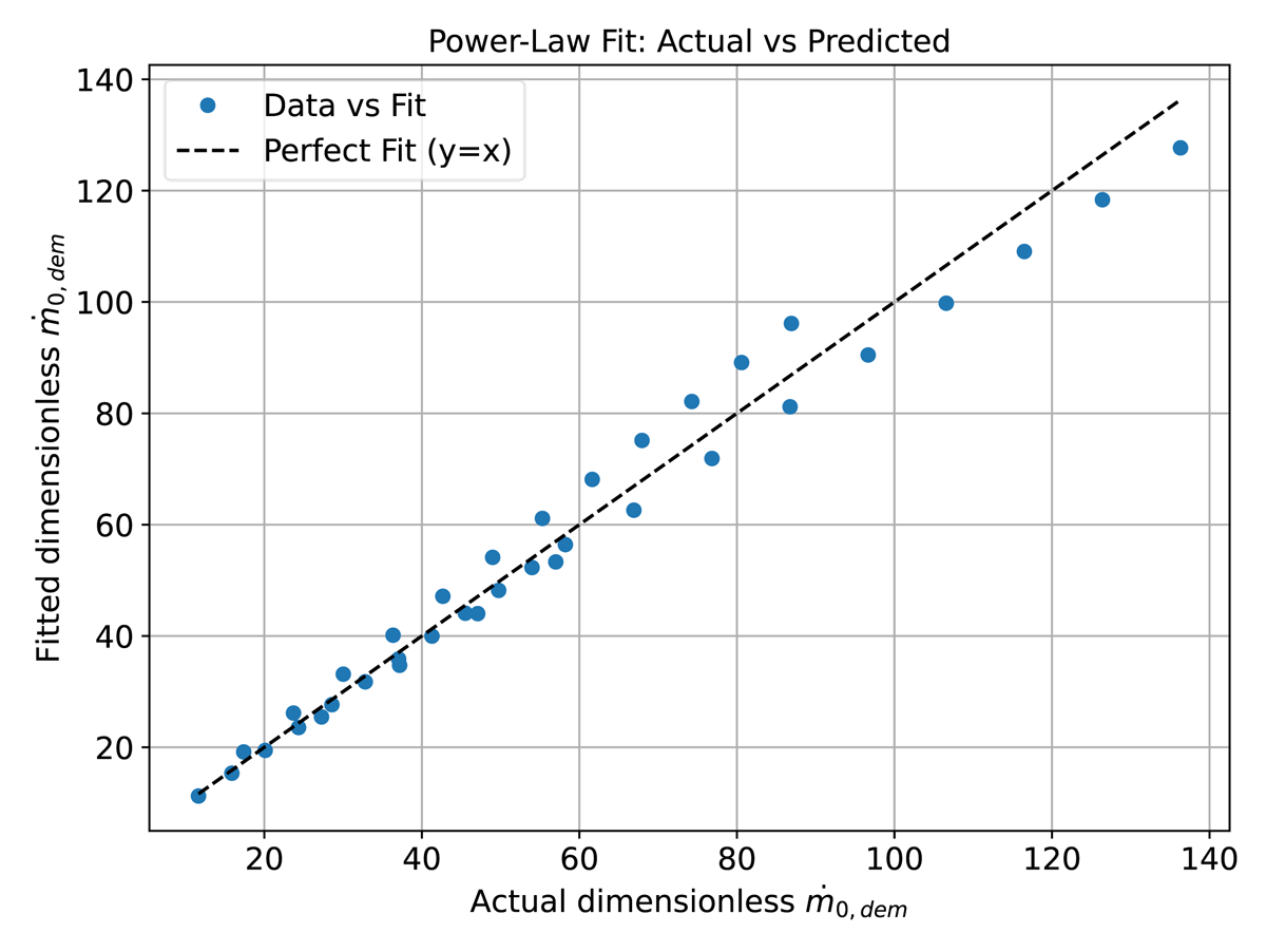
Figure 2
comparison between prediction and experimental data (Saury et al., 2005).
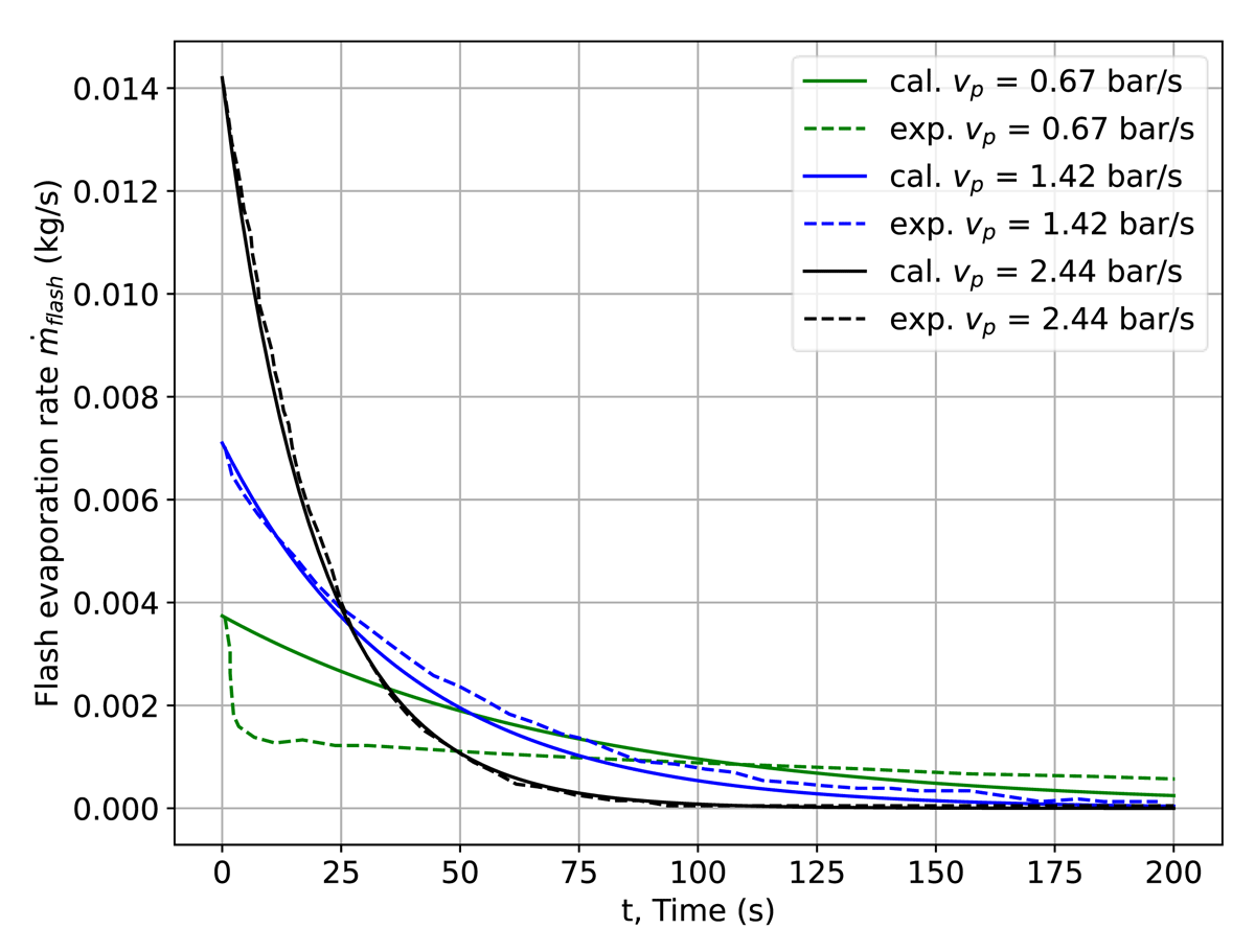
Figure 3
comparison between prediction and experimental data (Saury et al., 2005).
The experiment on liquid hydrogen flash evaporation in a pipe is being conducted as part of the ELVHYS project at KIT (Ustolin et al., 2023). The model will be updated based on the forthcoming experimental data.
Another consideration may be important. Bulk condensation in the vapor phase: When the vapor phase exists as a two-phase mixture (0 < quality <1), Machalek et al. (2021) suggests adjusting fluid densities to account for additional condensation mass (kg). However, we prefer modeling a bulk condensation rate (kg/s) instead, ensuring compatibility with the liquid and vapor mass conservation equations.
2.1.4 Wall-to-fluids heat transfer
The wall of the LH2 tank consists of an interior metal shell, a vacuum space with multi-layer insulation (MLI) material, and an external metal shell, as seen in Figure 4. The vacuum and low thermal conductivity of the MLI significantly reduce the heat transfer from the outside environment. In this model, the wall is divided into two parts, corresponding to the liquid and vapor phases, respectively. Each part is further subdivided into three nodes: the interior shell, the MLI layer, and the external shell.
where the heat flux is imposed at the wall-hydrogen interface (either convection or boiling), QW,α, and at the environment air-wall interface (convection), QEW,α, which serves as boundaries of the energy equation. The mass of wall mW,α varies with the liquid level. The heat capacity CW,α of wall depends on the wall temperature.
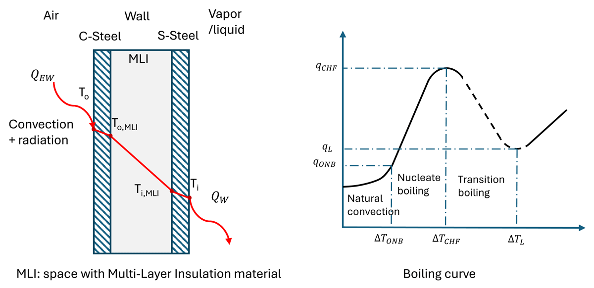
Figure 4
Illustration of heat transfer from wall to fluid.
In case of convection: The overall heat transfer rate (Daigle et al., 2011; Machalek et al., 2021; Osipov et al., 2011), , between the hydrogen at phase, α, and the wall is the sum of the heat transfer rate at the vertical surface (side wall) and the heat transfer rate at the horizontal flat surfaces (top and bottom) of the vertical tank. This approach can be converted for a horizontal tank using a tank geometry subroutine.
The heat transfer from air to wall follows the same methodologies as , using air temperature and properties, regardless of whether convection or boiling of liquid hydrogen occurs at the inner surface.
In case of boiling: Pool boiling occurs when the liquid reaches saturation conditions, and a temperature difference () exists between the wall and the liquid saturated temperature. This phenomenon acts as a secondary heat and mass transfer mechanism between the liquid and vapor phases. Pool boiling comprises four distinct regimes, as shown in Figure 4, with Table 1 summarizing the corresponding temperature ranges, heat transfer relationships, critical heat flux (CHF). Before introducing boiling, high heat flux scenarios cause excessive heating of liquid phase. This occurred because the liquid rapidly absorbed heat from the walls, while the evaporation rate—and the associated energy dissipation through the interfacial film—remained insufficient. Introducing boiling addresses this limitation by capturing the accelerated evaporation process. The boiling rate () is calculated as the ratio of heat transfer attributable to boiling to the latent heat of vaporization, assuming the liquid remains at saturation conditions:
Note: is the overall heat flux, and the convection flux should not be repeatedly added into in the boiling case. The film boiling regime was implemented, although the temperature difference (ΔT) is anticipated to remain below the film boiling threshold . However, it could exceed this threshold under abnormal scenarios (e.g. interior shell leak or engulfing fire). The theoretical heat flux expression of the boiling curve is documented in reference (Wang et al., 2016). , , and we fitted as a curve depending on pressure, instead of using a constant, as shown in Figure 5. Even using only four data points, the fitting provides a more accurate representation than employing a constant, as the range of is large and varies significantly with pressure.
Table 1
Hydrogen boiling regimes (Machalek et al., 2021; Wang et al., 2016).
| REGIME | ΔT (K) | q̇boiling (W/M2) |
|---|---|---|
| Natural convection (Shirai et al., 2010) | ||
| Nucleate boiling (Kutateladze, 1959) | ||
| Transition boiling (Carey, 2008; Zuber, 1959) | ||
| Film boiling (Breen and Westwater 1962) | |
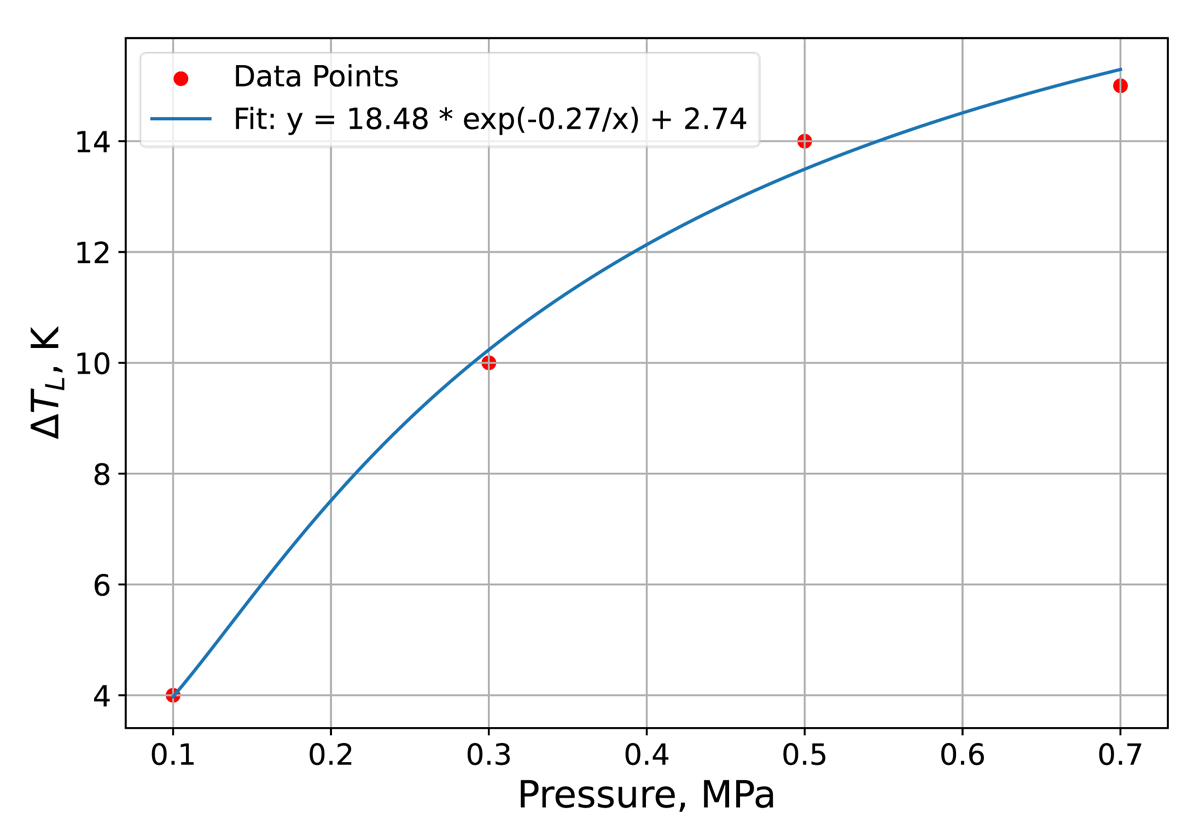
Figure 5
LH2 film boiling threshold vs pressure.
2.1.5 Conductivity of degraded MLI
Regarding the modeling of MLI degradation in case the tank engulfing in fire, a fully detailed model accounting for layer-by-layer degradation is highly complex. As referenced in studies (Camplese et al., 2024; Hajhariri et al., 2025), the degradation process is a progressive phenomenon dependent on the temperature profile through the MLI stack. In this work, which focuses on a system-level model of the entire LH2 tank, we have implemented a simplified yet physically representative approach. Our model captures the essential behavior of MLI degradation by defining effective thermal conductivity as a continuous function of temperature, transitioning from its pristine to a fully degraded state. The effective thermal conductivity, k(T), is given by a piecewise function with a transition region is governed by a power-law relationship:
where the lower limit (k0): the initial thermal conductivity of 0.00024 W/m·K represents the intact, non-degraded MLI under high vacuum; the upper limit (kmax): the maximum thermal conductivity of 0.2 W/m·K represents the MLI in a state of complete degradation, where the vacuum is lost and the layers are compromised. It equals roughly to thermal conductivity of the solid spacer material. The conductivity transitions between these two limits are based on a power-law function hypothetically. The transition begins at an onset temperature (Tonset = 500 K) and completes at a full degradation temperature (Tfull = 933 K). The exponent n = 2 controls the steepness of this transition. The exponent value was chosen as a representative, mid-range value that produces a physically realistic and numerically stable degradation profile. Experimental investigation is required to precisely quantify this exponent for specific MLI configurations under LH2 tank failure conditions. This parameter could be calibrated against such experimental data.
This formulation clearly shows the three distinct regimes of your model: the intact state, the progressive degradation transition, and the fully degraded state. This simplification allows the system-level model to account for the critical effect of insulation degradation under extreme heat loads (e.g., fire engulfment) without introducing prohibitive computational complexity from a detailed layer-by-layer analysis, which we agree is a valuable topic for future high-fidelity component-level studies.
2.2 Case studies and model setup
2.2.1 Validation cases: NASA MHTB and BMW experiments
Description of NASA MHTB Experiment
The validation of self-pressurization and pressure relief valve (PRV) release is based on experimental data from the NASA MHTB 50% fill level test (p263981t, 1998) (Hastings et al., 2003). In this self-pressurization test, the process continued until the vapor pressure reached the release valve threshold, with venting occurring throughout the procedure.
The MHTB aluminum tank is cylindrical, measuring 3.05 m in height and diameter, with a 2:1 elliptical dome. It has an internal volume of 18.09 m3 and a surface area of 35.74 m2, making it a reasonable representation of a full-scale space vehicle LH2 tank, as shown in Figure 6 left image. In this experiment, the initial liquid fraction was 50%, and the initial pressure was 111.2 kPa. The tank heat leak was measured at 51 W, but in the current calculations, heat transfer is determined using a model rather than this fixed value. The release valve operates between an upper limit of 137.9 kPa and a lower limit of 131.0 kPa, with a vent flow rate of 0.0048 kg/s, corresponding to an orifice diameter of 3.73 mm. The orifice dimension and set pressure were directly adopted from the specifications provided in the official experimental reports (Hastings et al., 2003). To ensure proper insulation performance, the vacuum chamber pressure was maintained at 10–6 torr or lower. For calculations, the initial liquid and vapor temperatures were assumed to be saturated. Additional details on the initial conditions can be found in reference (Hastings et al., 2003). Table 2 provides the material properties considered for tank shells and MLI.
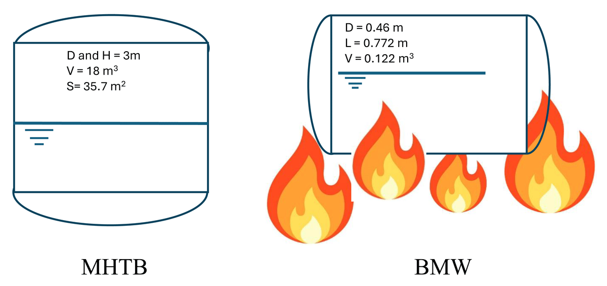
Figure 6
MHTB (vertical) and BMW (horizontal) experiment tanks.
Table 2
Tank walls & isolation properties (Ustolin et al., 2021).
| PARAMETER | INNER WALL, 5083 ALUMINUM | OUTER WALL, AISI 304 STEEL | MLI (VACUUM/AIR/ICE/DEGRADATION) |
|---|---|---|---|
| Thickness (m) | 0.003 | 0.003 | 0.035 |
| Specific heat, Cp (J/kg-K) | 897 | 490 | 1000 |
| Conductivity, 𝜅 (W/m-K) | 120 | 16 | 2.4E-4/2.2E-2/2.0E-1/Function (T) |
| Density, 𝜌 (kg/m3) | 2660 | 7800 | 45/45/100/45 |
Description of BMW Experiment
In the 1990s, BMW Group, in collaboration with Messer Griesheim GmbH and Linde AG, developed a double-walled LH2 tank for automotive applications (Pehr, 1996a and 1996b). Between 2005 and 2007, BMW produced the Hydrogen 7, a dual-fuel (hydrogen/gasoline) internal combustion engine vehicle equipped with an onboard LH2 storage system (BMW Group, 2025). Two tank designs were developed: one constructed entirely from austenitic stainless steel, and another featuring an austenitic stainless steel outer shell with a cold-tough aluminum alloy inner vessel (Pehr, 1996a). These tanks had a volume of 122 dm3 and were insulated using, specifically, 80 layers of multilayer insulation were installed within a 35 mm gap between the inner and outer shells.
As the Hydrogen 7 was the first consumer vehicle equipped with an LH2 storage system, BMW Group, in collaboration with tank manufacturers, licensing authorities, universities, scientific institutes, and the German armed forces, conducted a comprehensive four-year safety research program from 1992 to 1995 (Pehr, 1996b). Fire tests on the LH2 tanks, seen Figure 6 right, described in Pehr (1996a), were a critical component of this program. Both tank designs were tested, but only the results for the stainless steel-aluminum vessel are reported in Pehr (1996a). This study focuses on the stainless steel-aluminum LH2 vessel as well as in the refence (Ustolin et al., 2021), where we can find the detailed summary and analysis of the experiment.
In these experiments, the tanks were fully engulfed in a propane fire with an average flame temperature of 1193 K (Pehr, 1996a). The tanks were filled to approximately 55% capacity. PRVs were positioned outside the fire zone to prevent premature venting of evaporated hydrogen due to heat-induced leakage. The PRVs fully opened approximately four minutes after the test began. After 14 minutes, the entire LH2 content had evaporated. Subsequently, the aluminum inner shell began to melt, while the austenitic stainless steel outer shell withstood the fire for over one hour. Additionally, the pressure within the vacuum jacket increased significantly six minutes after the propane fire was ignited, and the vacuum was completely lost after four minutes. This loss of vacuum is expected to increase the thermal conductivity of the insulation.
The thermal conductivity of the MLI, estimated with temperature dependent function Equation 22 to model its degradation procedure in fire. It is noteworthy that the tank is oriented horizontally, requiring the use of a subroutine to update the tank geometry parameters over time by converting the liquid volume into liquid-vapor interface area, and wall area for accurate heat transfer calculations. Liquid hydrogen is maintained initially at saturated conditions at a pressure of 1 bar. The relief valve pressure settings are 4.14 bar (lower threshold) and 4.68 bar (upper threshold).
The minimum section of the relief valve is assumed to be 3 mm in diameter since no specific valve information was available in public literature. An initial simulation using a valve size 9.6 mm suggested in a prior modeling study (Ustolin et al., 2021) resulted in a significant discrepancy with the experimental data. Therefore, the valve size 3 mm was treated as a calibrated parameter and adjusted to match the measured pressure transients, ensuring the model’s accuracy for validation purposes.
2.2.2 Application case: KIT tank (AppLHy! project)
In the AppLHy! project a small container-based liquefier will be installed at the EnergyLab of KIT (Fuhry et al., 2025). The liquefier is connected to an LH2 tank, for which the loss-of-vacuum scenario—wherein the vacuum annulus is filled with air or ice—and an engulfing fire scenario involving MLI degradation is analyzed herein. The thermal conductivity, density, and heat capacity of air (see Table 2) are used to model the defective insulation layer. The LH2 tank is modeled as a vertical cylindrical structure with a diameter of 1 m and a height of 3 m. The tank has a total volume of 2.36 m3 and is assumed to be 50% filled with LH2. The relief valve is set to activate between 2.9 bars (lower limit) and 3.2 bars (upper limit), with an orifice diameter of 4 mm. The rupture disc opens at the threshold of 4 bar and orifice diameter 4 cm. The dimensions of PRV and rupture disc were obtained from the actual design specifications of the tank system. For the fire engulfment scenario, the PRV was explicitly sized 1 cm to handle the maximum expected gas generation rate. An appropriate orifice diameter was selected to provide this relief capacity at the designated set pressure.
During normal operation, characterized by the absence of vacuum loss in the multilayer insulation, the system’s boil-off rate is approximately 0.1–0.5% per day, equivalent to 0.167–0.84 kg/day/m3, which depend on the sun radiation heat and the area-volume ratio. For the design of a zero-boil-off LH2 tank, the results indicate the requisite cooling power for the integrated tank cooler.
3.0 Results and Discussion
3.1 Model validation against experimental data
3.1.1 Results for NASA MHTB case
Figure 7 compares the pressurization data from the MHTB experiment with the model predictions. The datasets show a clear trend of increasing pressure over time during the self-pressurization phase. The model closely follows the experimental data, demonstrating good agreement. The initial discrepancy can be attributed to the starting conditions of the test, as the self-pressurization test began at 10,380 s, suggesting the system had already reached a quasi-steady state. During valve operation, the model predicts a faster vapor pressure increase compared to the test data. However, the predicted pressure drop rate aligns reasonably well with the experimental data. The model predicts 15 pressure cycles, compared to the 10 observed in the test data. This suggests that the calculations assumed a larger heat transfer, which implies the need for a smaller thermal conductivity in the model. The thermal conductivity was identified as a key parameter influencing the cycle count. A series of simulations with varying conductivity values were conducted, demonstrating that the model’s output aligns with the experimental data only when a specific, lower value is used, thus justifying its selection. However, the pressurization time becomes longer in that case. In our simulation, the liquid tank is assumed to be in a saturated condition, whereas in the experiment, it might have been slightly subcooled. Unfortunately, we cannot determine the initial experimental conditions with high accuracy.
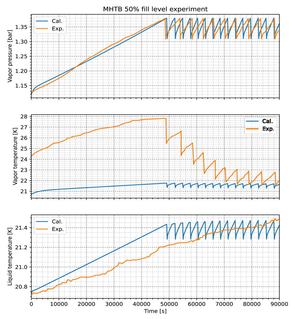
Figure 7
Compare with MHTB experiment.
The observed discrepancy in vapor temperature, particularly during the self-pressurization phase, is attributed to thermal stratification in the vapor phase. CFD results (Wan et al., 2023) show the vapor temperature increases with height, reaching up to 50 K in the upper regions. While the predicted liquid temperature aligns generally with the measured data, no fluctuations are observed in the measurements after the release valve is activated. This could be influenced by factors such as the area-to-volume ratio or the pressure threshold of the release valve, as indicated by the calculated liquid temperature in Figure 7. Additionally, measurement accuracy of experiment could be questioned, as it is almost impossible to have a 0.2 K precision at the concerned temperature level.
3.1.2 Results for BMW case
Figure 8 shows the comparison between the experimental measurements and the model results of the evolution over time of the pressure build-up, gaseous and liquid hydrogen temperatures, liquid hydrogen level inside the tank, and the inner and outer wall temperatures. The simulation results exhibited strong concordance with experimental pressure measurements. Specifically, the initial opening of the PRV was predicted at around 350 seconds, closely aligning with the observed time during fire tests. Furthermore, the pressure relief valve remains open for over 8 minutes following a specific time point, subsequently exhibiting low-frequency fluctuations. These pressure phenomena arise from variations in heat transfer, driven by changes in the contact area and the balanced release of gaseous hydrogen mass. However, a 15% deviation persists in the liquid level, with the liquid level sensor recording the minimum level at 900 seconds. This discrepancy may be attributed to the valve diameter of 3 mm, which is potentially undersized compared to the 9.6 mm valve diameter used in the reference simulation (Ustolin et al., 2021). Conversely, the model’s temperature predictions could not be validated against experimental measurements, as illustrated in Figure 8, which is also quite like the results from (Ustolin et al., 2021). This discrepancy is particularly evident for gaseous hydrogen and inner shell temperatures. The precise locations of the measurement points within the tank during testing are unspecified, and interpreting the temperature data from (Pehr, 1996a) is challenging due to the broad temperature range (0–1400 K) used in the graphical representation. It is evident that the MLI decomposes within minutes at environmental temperature of approximately 1200 K. Wall boiling predominantly governs the wall heat transfer. Nevertheless, no rupture disc activation occurred, indicating that the relief valve design is safe.
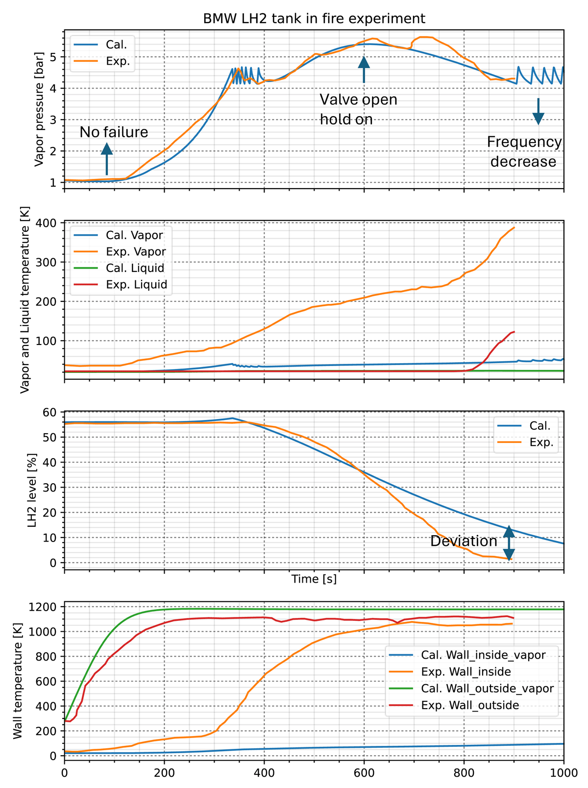
Figure 8
BMW LH2 tank behavior in fire.
3.2 Analysis of tank vacuum loss scenarios (KIT tank)
3.2.1 Loss of vacuum scenarios
One quasi-realistic failure mode for cryogenic storage tanks is the loss of vacuum within the insulation layer between the inner and outer metallic shells. In this scenario, the vacuum gap is assumed to be replaced by air or nitrogen ice. Consequently, the thermal conductivity of air or nitrogen ice are adopted for analysis, while the density and heat capacity values of the original insulation layers (see Table 2) are retained to represent the multilayer insulation.
Vacuum gap replaced by air
Figure 9 illustrates the behavior of the tank when the vacuum gap is replaced with air, which exhibits a thermal conductivity approximately 100 times greater than that under nominal heat transfer conditions. The left frame of Figure 9 highlights the first around 1.4 hours of hydrogen boil-off, showing the evolution of mass loss. In this regime, hydrogen is vented through a pressure relief valve, ensuring the tank is safe under vacuum loss accidents. The temporal evolution of liquid and wall temperatures indicates a gradual increase over time. As the liquid warms, its density decreases slightly, which results in a small rise in liquid level during the pressurization phase.
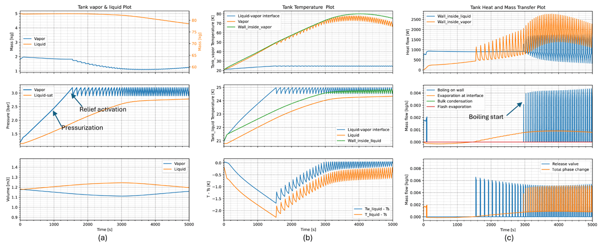
Figure 9
AppLHy! tank parameters when vacuum loss and the space replaced by air.
Figure 9b shows the temporal evolution of liquid, vapor, and inner wall temperatures. The vapor temperature oscillates with the relief valve operation. At approximately 3000 seconds, the vapor temperature oscillates faster while the liquid temperature remains comparatively stable. The wall temperature on the liquid side approaches the saturation temperature, marking the onset of boiling. The onset of boiling enhances phase-change mass transfer, with the mass flux governed by the finite heat flux through the MLI. This also leads to faster pressure fluctuations compared to those observed during the initial activation of the pressure relief valve. Such rapid valve cycling may increase the risk of mechanical failure.
The corresponding mass flow and heat transfer are depicted in Figure 9c. The dynamics reveal consistent predictions of the tank’s behavior, as reflected by the timing and frequency of venting. When the relief valve opens, the rapid reduction in vapor pressure triggers immediate evaporation—and, in the later phase, boiling—of the liquid phase to restore thermodynamic equilibrium. Consequently, a larger quantity of hydrogen vapor is vented before the pressure decreases to the 2.9 bar closing threshold. The dynamics provided that the relief valve operates reliably, the tank pressure can be safely maintained below 3.2 bar.
Vacuum gap replaced by N2 ice
When the vacuum integrity of a liquid hydrogen storage vessel is compromised, residual atmospheric gases penetrate into the evacuated annular region and undergo cryogenic condensation and solidification on the cold inner wall. Although oxygen possesses a higher condensation temperature than nitrogen, nitrogen preferentially forms solid deposits because its melting point (63 K) exceeds the local wall temperature, whereas oxygen, with a lower melting point (54 K), initially remains in the liquid or vapor phase until further thermal equilibration occurs. Here, we assume that only nitrogen ice replaces the vacuum space, with a relatively large effective thermal conductivity of approximately 0.2 W/m·K.
Figure 10 illustrates the scenario of vacuum loss where the insulation gap is replaced by solid nitrogen. The PRV activates after approximately 105 seconds, which is significantly earlier than in the case of air replacement. Following a brief pressure decrease, the tank pressure rises again until the rupture disc opens at vapor pressure 4 bar. This behavior clearly indicates that the PRV discharge cannot compensate for the accelerated hydrogen boil-off, which is driven by the high effective thermal conductivity of the nitrogen ice layer.
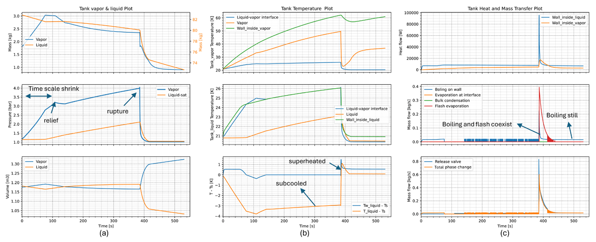
Figure 10
AppLHy! tank parameters when vacuum loss and the space replaced by N2 ice.
After the rupture disc opens, the release mass flow becomes sufficiently large that the tank pressure decreases sharply. This rapid depressurization is reflected in the temperature profiles, where the liquid hydrogen is observed to be subcooled prior to rupture and superheated immediately afterward. The two-phase change curves further demonstrate that flash evaporation occurs as a result of the sudden pressure drop and the subsequent liquid superheating. The flash evaporation mass flow is represented by a decay function, consistent with the model assumptions, with an initial peak of approximately 0.4 kg/s, which clearly dominates the two-phase heat and mass transfer. After approximately 45 seconds following the rupture disc activation, the flash process ceases as the superheat falls below the threshold of 0.1 K. At this stage, however, nucleate boiling at the liquid-wall interface persists and becomes the dominant heat transfer mechanism in the later phase.
3.2.2 Engulfing Fire Scenario
A second quasi-realistic scenario investigated corresponds to exposure of the storage vessel to elevated external temperatures, representative of conditions that may arise during an external fire. In this case, the ambient environment surrounding the hydrogen tank is assumed to be at 1200 K. This value represents a conservative upper bound (worst-case assumption) for temperatures reached in standardized bonfire tests (Pehr, 1996a and 1996b). The analysis accounts for convective heat transfer and radiative contributions from the fire. Furthermore, the boundary condition assumes a uniform ambient temperature around the entire tank surface, rather than localized heating from one side. Under fire or high-temperature exposure, the thermal performance of MLI progressively degrades as rising temperature increases the effective thermal conductivity. This degradation spans from partial loss-of-vacuum, where conductivity gradually increases, to full failure characterized by vacuum loss and melting of spacer materials, resulting in maximum heat transfer to the tank. The thermal properties—thermal conductivity (assumed to be a temperature-dependent function), density, and heat capacity, as listed in Table 2—are applied to the middle wall layer. Such a condition may arise if fire-induced damage compromises the tank insulation. In this run, the PRV was configured with a diameter of 1 cm to investigate the dynamics of tank behavior and test the tank design.
The results for the fire exposure scenario, as shown in Figure 11, demonstrate behavior qualitatively like that observed during insulation failure in the BMW experiment. The pressure evolution is characterized by a sharp increase in several minutes in the beginning because of the MLI decomposition, and then by cyclic opening and closing of the PRV, with a period of opening time comparable to that observed in the experiment. A stable PRV operation is not achieved, and the rupture disc does not activate. In the case of fire exposure, approximately half of the liquid hydrogen boiled off within 15 minutes, resulting in a rapid release of hydrogen gas. Figure 11b illustrates the temporal variation in temperatures, highlighting cyclic temperature fluctuations in the liquid phase. Notably, the temperature difference (ΔT) between the liquid saturation temperature and the inner wall is maintained at around 1 K post-PRV activation, influencing heat transfer dynamics. This temperature difference triggers nucleate boiling at the liquid–wall interface when ΔT exceeds 0.1 K. Boiling facilitates mass transfer from liquid to vapor, with wall boiling dominating the two-phase transition, as depicted in Figure 11c.
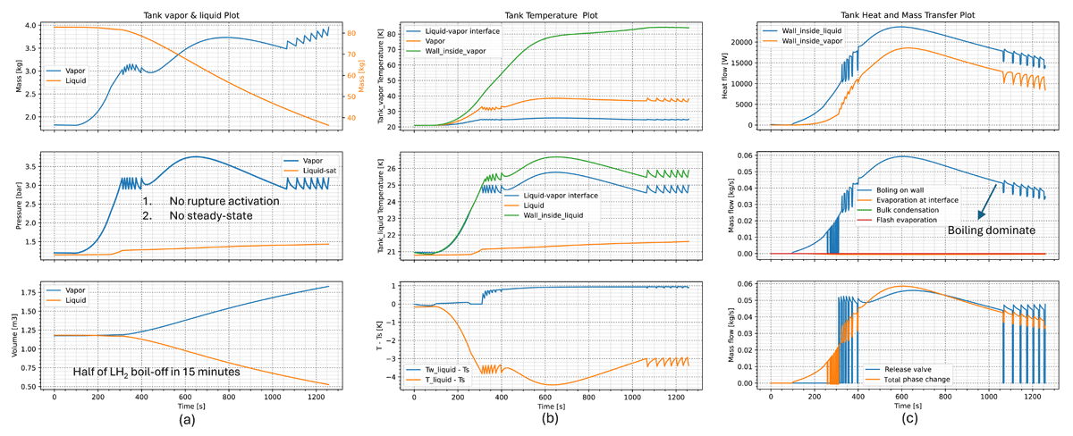
Figure 11
AppLHy! tank parameters when MLI degradation in fire.
Figure 11c shows the absence of significant flashing during the engulfing fire scenario with degrading MLI, which appears like the loss-of-vacuum case: vacuum gap replaced by air, is primarily due to the different pressure dynamics governed by the PRV sizing. In the engulfing fire case, a larger PRV (diameter = 1 cm) was used to test the tank’s ability to maintain pressure under extreme conditions. This larger orifice provides sufficient venting capacity to handle the boil-off gas generated by the fire, preventing a rapid pressure drop that would trigger flash evaporation. In contrast, the loss-of-vacuum case used a smaller PRV (diameter = 4 mm). This smaller orifice creates a higher flow resistance. If this smaller PRV were used in the fire scenario, it would be undersized and unable to vent the high boil-off rate, leading to an overpressure that would activate the rupture disc. The subsequent rapid depressurization through the rupture disc would then indeed cause flashing, like the loss-of-vacuum case: vacuum gap replaced by N2 ice.
4.0 Conclusion
This study investigates the thermal response and dynamic behavior of LH2 tanks under vacuum loss conditions. A non-equilibrium lumped parameter model is developed to simulate boil-off dynamics, heat transfer, and blowdown rates, incorporating convection, various boiling regimes, and flash evaporation.
The LH2 tank is modeled as a two-node system representing liquid and vapor phases, with mass and energy balances governed by a comprehensive heat transfer framework. The approach integrates components from HyRAM, and CoolProp for thermophysical properties, enabling accurate predictions of hydrogen behavior during storage and pressure relief valve or rupture venting. Model validation against NASA MHTB and BMW experimental data for normal boil-off and accident in fire scenarios demonstrate good agreements, effectively capturing the trends of increasing pressure and temperature during self-pressurization and pressure evolution when MLI degradation, as well as the relief valve’s role in pressure control. A key advancement in the model development is the formulation and validation of a novel correlation for flash evaporation induced by a pressure drop within the tank, corroborated using experimental data from water flash tests. This model employs a time-dependent decay function, which aligns closely with experimental observations.
In the AppLHy! project, a loss of vacuum scenario and an engulfing fire scenario were analyzed for a liquid hydrogen tank connected to a small container-based liquefier at KIT’s EnergyLab. The LH2 vertical cylindrical tank, 50% filled, was modeled with a pressure relief valve activating between 2.9–3.2 bar (4 mm orifice) and a rupture disc opening at 4 bar (4 cm orifice). In the vacuum loss scenario, replacing the vacuum gap with air or nitrogen ice significantly increased thermal conductivity, leading to accelerated hydrogen boil-off. Air replacement caused cyclic PRV operation with pressure fluctuations, while nitrogen ice replacement triggered rapid boil-off, activating the rupture disc after ~105 seconds due to the PRV’s inability to manage the pressure rise, followed by flash evaporation and sustained nucleate boiling. In the fire exposure scenario (1200 K ambient temperature), multilayer insulation degradation increased heat transfer, resulting in rapid LH2 boil-off (~half LH2 in 15 minutes) with cyclic PRV operation but no rupture disc activation. Temperature profiles showed liquid superheat of ~1 K post-PRV activation, driving nucleate boiling at the liquid–wall interface (if ΔT > 0.1 K), which dominated two-phase mass transfer, consistent with BMW experiment insulation failure dynamics.
The findings provide critical insights into the behavior of LH2 tanks under loss-of-vacuum and fire exposure scenarios, yet several areas warrant further investigation to enhance the accuracy and applicability of the models. A primary focus for future work is the improvement of the flash evaporation model, building on experimental data from the ELVHYS project. This involves refining the representation of two-phase mass transfer dynamics, particularly the flash evaporation process triggered by rapid depressurization following rupture disc activation, to better capture the transient behavior observed in the experiments. Validation efforts must continue at both the system level (tank dynamics) and the specific model level (heat transfer mechanisms), ensuring that simulations align closely with experimental outcomes. Specifically, for the fire exposure scenario, the influence of fire coverage and the degradation of MLI remain critical areas of interest. Developing a comprehensive model for MLI degradation under varying fire intensities and coverage patterns will be essential to accurately predict heat transfer rates and their impact on tank pressure and boil-off behavior. These advancements will enhance safety, addressing the challenges posed by extreme conditions such as insulation failure and external fire exposure.
Data Accessibility Statement
The data and model code that support the findings of this study are available from the corresponding author upon reasonable request.
Acknowledgements
The authors express their gratitude to the project partners of the TransHyDE project AppLHy! for their excellent collaboration on topics related to the transport and application of liquid hydrogen.
Competing Interests
The authors have no competing interests to declare.