
Nomenclature
| A | Area in m2 | lf | Flame length in m |
| ap | Planck-mean absorption coefficient | p | Pressure in bar (absolute) |
| C* | Non-dimensional radiant power | Qrad | Thermal radiation in W/m2 |
| df | Flame diameter in m | Re | Distance between radiation sensor and point source in m |
| D | Outlet diameter in m | Rs | Vertical distance between radiation sensor and release point |
| f | Frequency in 1/s | SEP | Surface emissive power in W/m2 |
| fs | Stochiometric mass fraction fuel | t | Time in s |
| ΔHc | Lower heating value in MJ/kg | T | Temperature in °C |
| Maj | Mach number in the expanded jet unitless | uj | Exit velocity of the expanded jet in m/s |
| ṁ | Mass flow in kg/s | uw | Wind velocity in m/s |
| N | Number of point sources | xRAD | Radiant heat fraction unitless |
| L | Length in m | x,y,z | Coordinates in m |
| Greek | |||
| λ | Wavelength in µm | ϕ | View Factor unitless |
| ρf | Density of the flame in kg/m3 | τ | Transmissivity unitless |
| ρ0 | Density of cold fuel in kg/m3 | τR | Residence time in ms |
1. Introduction
In the transition from fossil fuels to renewable energy sources, hydrogen is expected to play a decisive role. The versatility of hydrogen as an energy carrier enables a wide range of applications in the chemical industry or in the energy sector. However, appropriate safety measures have to be implemented to ensure a safe use of hydrogen, especially in production, transportation and storage. These need to be derived from a hazard assessment that quantifies the risk of consequences. One possible scenario is the release of hydrogen due to a leakage in pipelines, flanges, or storage containers. A potential risk to be considered is the momentum driven release into the environment because hydrogen is typically stored under high pressure. Another technical scenario is the momentum driven release through safety valves and/or blow off pipes. Due to the low ignition energy of hydrogen and its potential for self-ignition or ignition by external ignition sources, a diffusion jet flame can occur (Gummer, 2008). Parameters such as the flame geometry and the emitted thermal radiation to the environment need to be characterized to validate jet flame models that are used for hazard assessment purposes.
The first experimental studies on diffusion jet flames were carried out at the beginning of the 20th century by Burke and Schumann (1928). Based on experimental data, analytical formulas and models were derived to characterize diffusion flames of cylindrical shape. Based on this, subsequent investigations of turbulent diffusion flames were performed by Hawthorne, Weddell and Hottel (1948) who observed correlations between the flame length, nozzle diameter and the Froude number. Bilger (1976) investigated the relation between diffusion flame structure and the reaction rate of oxidizer and fuel. Correlations between density gradient, turbulent mixing and species concentration were identified. Most of the hydrogen jet flame models that are currently used are based on experimental data by Shevyakov and Komov (1977), Becker and Liang (1978), and Kalghatgi (1984), who did fundamental research on the flame geometry of diffusion jet flames. They established dependencies on the outlet diameter, mass flow, Froude Number, Reynolds number, and the resulting visible flame length. Based on these data, Molkov and Saffers (2013) developed a model, taking into account the fluid-mechanical properties, in which the dimensionless flame length can be represented as a function of the outlet fuel density, density of surrounding medium and Mach number.
When looking at the experimental data in the literature, it becomes apparent that there is no standardized description and procedure for determining the flame length. In particular, the point at which a boundary is drawn between ‘flame’ and the ‘surroundings’ is not uniformly defined. It is unclear, in particular, whether the ‘flame’ is limited to the reaction zone or also includes hot flue gases. In contrast to hydrocarbon flames, hydrogen flames do not emit significant radiation in the visible wavelength spectrum (cf. Figure 2). Studies by Gore, Jeng and Faeth (1987), and Schefer et al. (2009) have shown that hydrogen diffusion flames emit in a spectrum with a peak at 0.315 µm (OH*) and 1.8 µm, 2.7 µm, 4.3 µm and 6.3 µm (H2O). The determination of the visible flame length based on luminescence is therefore difficult, although it has been done in experimental studies. Here, the measurement of the flame length with low luminescence is only possible under darkened ambient conditions (Studer et al., 2009; Proust, Jamois and Studer, 2011) or with injection of luminescent components (Mogi, Nishida and Horiguchi, 2005; Imamura et al., 2008). In the latter case an influence on the flame shape and combustion behavior cannot be fully excluded. An investigation to determine the flame length using various measurement techniques such as luminescence, IR and OH* intensities was carried out on a laboratory scale by Schefer et al. (2006). The investigations showed that the type of measurement technique used has a major influence on the flame length results. It was found that the jet flames have the following morphology in terms of flame lengths: lIR > lVIS > lOH*.
Most studies on jet flame geometry, especially flame length, are based on laboratory-scale experiments with constant ambient conditions for horizontal or vertical outlet directions. In reality, atmospheric conditions such as wind can be expected to have an influence on flame geometry. To obtain a more realistic database for hazard assessment, large-scale experiments with inclined hydrogen jet flames (45° outlet angle) were carried out in the open field under constant outlet conditions. These experiments were performed at the Test Site Technical Safety of the Bundesanstalt fuer Materialforschung und -pruefung (BAM TTS). Results from this study, such as the flame geometry and radiant heat fraction, are discussed and compared to literature data and radiation models.
2. Methodology
2.1 Experimental Setup
Hydrogen is supplied from 6 bundles at a maximum pressure level of p = 300 bar each. This type of hydrogen supply allows constant outflow for durations of t >= 60 s for any of the investigated mass flows, ensuring quasi-stationary outflow boundary conditions. The outgoing fluid is passed through a manifold pipe and regulated using a control valve combined with a Coriolis mass flow meter (Rheonik Coriolis RHE28). Temperature and pressure sensors are installed along the pipe. A diffuser with a diameter of D = 30 mm is installed at the outlet of the outgoing pipe (L = 1 m). The diffuser is oriented in an outlet angle of 45° to the XZ plane (cf. Figure 1). After the hydrogen jet is released, it is ignited via a propane pilot flame. Following successful ignition of the jet, the pilot flame is switched off immediately (Bernardy et al., 2024).
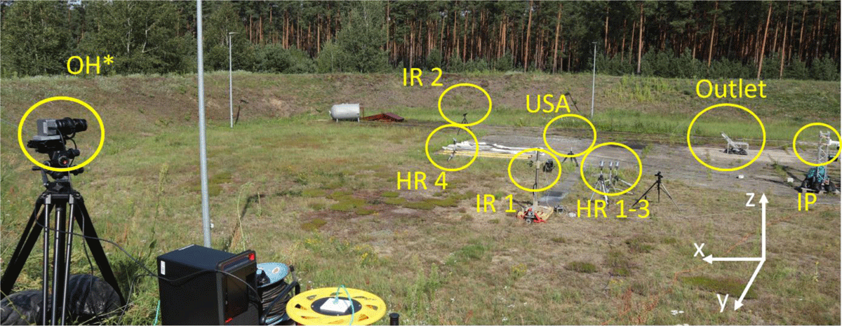
Figure 1
measuring equipment in free field at the test area.
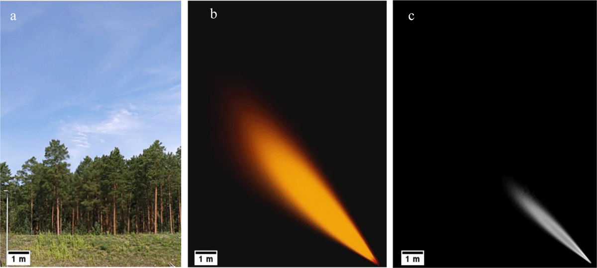
Figure 2
Comparison of the recording of a hydrogen jet flame with digital camera (a), time averaged IR camera (b) and time averaged OH* camera (c). The hydrogen flame is not detectable by visible light in open field conditions. The flame lengths estimated by IR and OH* measurements significantly differ.
To measure the thermal radiation emitted by the jet flame into the environment, four thermal radiation sensors (bolometers – Medtherm Series 64) are used. Three of these bolometers (cf. Figure 1 – Heat Radiation (HR) sensors) are directed towards the flame and are positioned at different distances. The fourth one is used to measure the background radiation of the environment and thus is directed away from the flame (cf. Figure 1-HR4). The background radiation is subtracted as an offset from each signal of the three HR sensors. The thermal radiation sensors operate within a wavelength spectrum of λ = 0.5 µm – 14.5 µm with a recording frequency of f = 100 Hz. They are designed to measure a maximum irradiance of Qrad = 2.25 kW/m2. Each sensor has a view angle of 55°. The latter defines the minimum distance between flame and sensor to ensure that the whole flame is covered. The minimum distance between sensor and flame must also take the maximum detection limit of heat radiation for the sensors into account. The positions of the radiation sensors (cf. Table 1) were selected according to the specifications mentioned above. Positioning the sensors one behind the other aimed at recording (three) independent heat radiation values for one test, ideally enhancing the quality of the results. For additional test monitoring, a swivelling 360° IP camera (BASCOM – 1 Dom System Plus; cf. Figure 1 IP) was installed. An overview of the positions of cameras and heat radiation sensors at the test areas is listed in Table 1.
Table 1
Position of measurement equipment in the open field.
| POSITION OUTLET NOZZLE (0|0|0) | IR 1 | IR 2 | OH* | IP | USA | HR1 | HR2 | HR3 | HR4 |
|---|---|---|---|---|---|---|---|---|---|
| x in m | 6 | 0 | 0 | –2 | 8 | 3.46 | 3.46 | 3.46 | 6.5 |
| y in m | 18 | 17 | 34 | 8 | 11 | 12.31 | 14.31 | 16.61 | 11 |
| z in m | 0,47 | 0,6 | 2 | 0,6 | 0.5 | –0.26 | 0.16 | 0.34 | –0.26 |
These positions are calculated considering the outlet of the nozzle as the origin of a Cartesian coordinate system, whose axis orientations are shown in Figure 1. For wind recording, an ultra-sonic anemometer (USA – Metek type USA-1 Scientific) is used. Moreover, the ambient temperature and relative humidity were measured for each test.
The flame geometry was determined with two IR camera systems. One camera is a FLIR SC4000 (cf. Figure 1– IR1) with cooled IR sensor, detecting a wavelength spectrum of λ = 1.5 µm – 5 µm and with a recording frequency of f = 50 Hz. The second IR camera, a FLIR A655 (cf. Figure 1 – IR2) has a wavelength of λ = 7.5 µm – 14 µm and a recording frequency of f = 50 Hz. As shown in Figure 1, these cameras are positioned with an angle offset of 90° in the XY plane to the release location so that the flame is captured from 2 perspectives. An EHD CMOS (EHD SCM9701-UV) camera was used to record OH* chemiluminescence images at f = 20 Hz. The camera is equipped with a 50 mm (EHD UV5035 B) lens transmitting in the UV range. The lens is used with a bandpass filter centered at 0.307 µm with a bandpass of 10 nm. The camera acquires each image with an exposure time of 0.2 seconds per image.
2.2 Experimental Program
A total of 36 experiments were performed. The whole test series covered a systematic investigation of mass flow rates ranging from ṁ = 0.0125 kg/s to ṁ = 0.175 kg/s.
In the following, the entire mass flow range is used for the consideration of the flame geometry. For consideration of the thermal radiation jet flames only with mass flows greater than ṁ > 0.05 kg/s (Ma > 0.6) are used. In the case of jet flames with lower mass flows, the measured thermal radiation at the position of the radiation sensors is below the lower calibrated measurement limit, which is why they were not taken into account for further evaluation.
3. Results and discussion
The main purpose of the investigations is to quantify parameters such as the flame geometry and the heat radiation emitted by an inclined jet flame. In particular, the determination of radiant energy released over the flame surface is sought. This parameter is referred to as the Surface Emissive Power (SEP). As this parameter cannot be measured directly, it needs to be inferred by measuring auxiliary quantities in various steps. The first auxiliary quantity that has to be determined is the flame geometry. Despite the constant outlet mass flow, the test conditions are only quasi-stationary over time due to the ambient conditions in the free field, in particular unsteady wind conditions. This results in fluctuations in the flame shape. To obtain a quasi-stationary flame shape nonetheless, the IR and OH* recordings are divided into single frames. These transient snapshots are then used to compute time-averaged flame shapes over the entire duration of each experiment, thus delivering mean values of the flame as shown in Figure 3. The flame shape (contour) is then defined via a RBG value, manually specified so that only the flame surface and no reflections from the test devices or the ground are visible in the image.
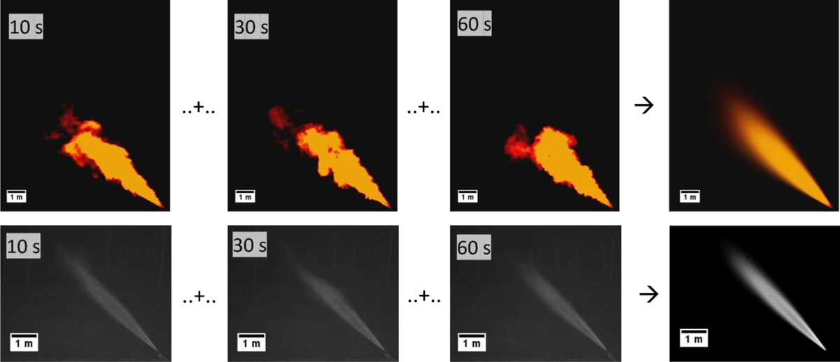
Figure 3
Schematic overview of averaging the individual IR (top line) and OH* (bottom line) images to generate a times average (stationary) flame image over the test duration.
The experimental results for the mean flame length of hydrogen, determined with an IR and OH* camera, are shown as a function of the Mach number in Figure 4. Here, Maj is the Mach number of the expanded jet, calculated according to Yüceil et al. (2002). The IR flame lengths show higher values in comparison with those determined with the OH* camera. These observations can also be found in Schefer et al. (2006). One reason for this result is that the IR camera records the whole wavelength of radiating particles. This includes preheated educts, reaction zone and hot exhaust products. A temperature of T >= 850 °C was selected for the IR camera to determine the flame boundary and visualize the jet flame. In contrast to this, the OH* camera focuses on the UV wavelength range of 0.302 µm to 0.312 µm. Within this wavelength, the OH* camera detects the electromagnetic radiation (hv) emitted by decaying OH* radicals. This reaction takes place in the combustion zone of the hydrogen flame and is mainly characterized by the two following reaction paths according to Schefer et al. (2006):
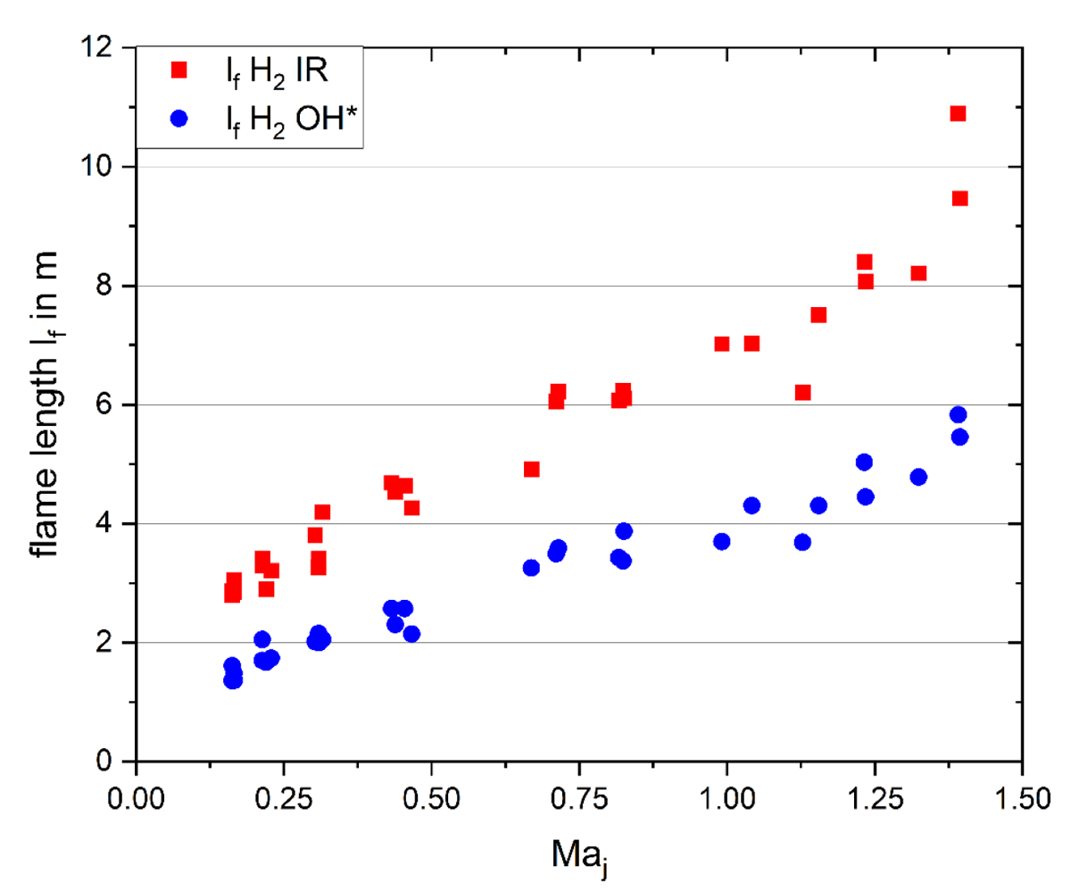
Figure 4
Comparison of hydrogen flame length determined by IR and OH* camera over the outlet Mach number Maj.
In Figure 5a, the ratio of the experimental flame lengths lf OH*/lf IR is shown to illustrate the differences between OH* and IR flame length measurement. The flame length ratio observed between OH* and IR is in the range of 0.62 to 0.47, thus the OH* flames are shorter than the IR flames. Data available in the literature show a similar trend. Schefer et al. (2006) investigated vertical hydrogen jet flames with OH* and IR cameras. Although an angle of 45° was investigated in the work presented here, the data of Schefer et al. are the only available data for comparison known to the authors and are deemed suitable for a phenomenological comparison. These investigations reveal that the flame lengths determined by OH* are shorter than those determined by IR, with a flame length ratio ranging from 0.85 to 0.75. Additionally, Schefer et al. observed a decreasing flame length ratio with increasing Maj (cf. Figure 5b). In the presented work, the flame length ratio shows no clear increasing or decreasing trend over the Mach number range investigated. Only the spread width (deviation between experimental values) decreases with increasing Maj. Differences in the absolute ratio values between the literature and the experiments in this work can be explained by the different outlet directions of 90° for the data of Schefer et al. and 45° in the presented experiments, since the outlet direction has a direct influence on the flame length due to different buoyancy effects.
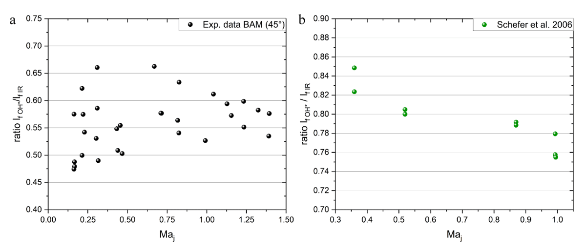
Figure 5
Comparison between experimental determined ratio of flame length OH*/IR (a) and the ratio of flame length OH*/IR by Schefer et al. (b) shown over the outlet Mach number Maj.
The decrease of the spread width for the experimental data in this work, might also be due to the influence of the ambient wind. For the low momentum range (low Maj) a large deviation (spread width) is present, which is reduced with increasing Mach number. As the flame shape is more sensitive to ambient wind when the outflow velocity is low (corresponding to low momentum regime as only one single outlet diameter was investigated, resulting in a single outlet velocity corresponding to each mass flow) the decrease in spread width can be explained with increasing outlet velocity.
To investigate the influence of the ambient wind on the flame, the ratio of the mean flame diameter to the flame length (df/lf) is used as an indicator for the compression of a jet flame. It represents the variation of the flame length with wind influence that leads to generally shorter but thicker flames. The higher the ratio, the more compressed the flame. In Figure 6, df/lf is plotted against the ratio of the wind velocity uw to the expanded outlet velocity uj. As the wind speeds observed in all experiments ranged from 1 m/s to 4 m/s and the observed outlet velocities ranged from 220 m/s to 1730 m/s, it can be deduced that decreasing values of the ratio uw/uj are mainly due to an increase of the outlet velocities (corresponding to increasing momentum as mentioned above) since the wind velocities are lower than the outlet velocities by several magnitudes. It is evident that the IR determined (df/lf) ratio shows a larger increase over the measured wind/outlet velocity range than the values determined with OH*. It can be deduced that OH* measurements are less sensitive to external parameters, such as the ambient wind, than IR measurements where a clear compression of the flame (shorter but thicker shape) can be observed with increasing wind. The OH* measurement focusing on the reaction/combustion zone of the flame visualizes a high momentum flow regime. Compared to this, the IR measurement visualizes every emitting region of the flame, from the combustion zone to hot flue gases. Since the momentum flux decreases along the flow region due to expansion in the surrounding medium, the corresponding momentum for the hot flue gases is much lower than in the combustion zone. With decreasing momentum the wind influence increases, impacting the flame region covered by the IR recording.
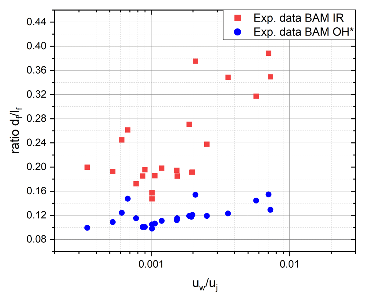
Figure 6
Comparison of ratio flame diameter to flame length for OH* and IR plotted over the ratio wind velocity to outlet velocity.
The main objective of the investigations was to experimentally quantify the thermal radiation emitted by jet flames. The amount of heat radiation that is released from the combustion of a fuel is described by the radiant heat fraction (xRAD). Since neither the radiant heat fraction nor the absolute heat flux in the flame can be measured directly, they must be derived from other measurable values. From the measured incident heat flux at the bolometers, the corresponding SEP of the flame can be calculated, and from this value the radiant fraction can then be derived. The SEP describes how much radiation energy is released in total over the flame surface during combustion. The SEP can be derived from the measured heat radiation at the bolometers (cf. Table 1) using Eq. (1) (Chamberlain, 1987; van den Bosch and Weterings, 2005):
The geometric ratio of the flame shape to the bolometer view field is described by the view factor ϕ1_2. The index ‘1_2’ refers to the path between emitter ‘1’ and receiver ‘2’. Frequently used analytical approaches that model the flame as a cylinder can be found in the literature (VDI, 2010). For more complex flame shapes and angles between emitter and receiver, as the ones investigated here, a suitable analytical approximation is not available. In this work, a numerical method was developed to determine the view factor. The flames are divided into slices (with one pixel width) corresponding to a ‘disc’ of the flame body, when assuming a rotational symmetry of the flame. The view factor is then calculated for each slice and integrated across the flame contour. The transmittance τ in Eq. (1) is calculated according to Wayne (1991), and is based on the measured ambient temperature and relative humidity for each test. The experimental results for the SEP over the Mach number are shown in Figure 7a. The calculated SEP of OH* and IR differ by a factor of 5 to 6. This is due to the different flame sizes recorded by the IR and OH* imaging (cf. Figure 7b) and subsequently differences in the view factor of the flame used to calculate the SEP (Eq. 1).
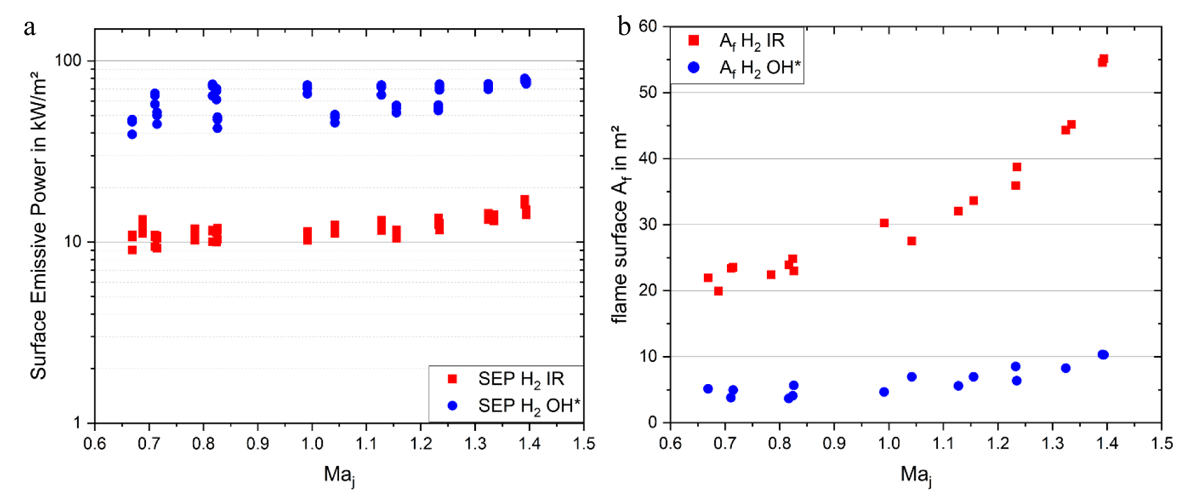
Figure 7
Comparison of (a) Surface Emissive Power and (b) flame surface area of hydrogen jet flames determined using IR (red) and OH* (blue), results are plotted against the expanded outlet Mach number, Maj.
Based on the SEP, the characteristic parameter xRAD can be derived. The parameter can be calculated according to Eq.(2) using the experimentally determined values for SEP and Aflame shown in Figure 7.
Figure 8 illustrates the radiant heat fraction values for OH* and IR, calculated according to Eq. (2). Unlike the SEP, the radiant heat fraction remains independent of the measurement technique used (OH* showing the same values as IR). It can therefore be concluded that for the purpose of determining the radiant heat fraction (only) there is no apparent dependency of the measurement technique used in these experiments. The variation in the recorded flame dimensions is fully compensated by the view factor, leading eventually to comparable results, proving the consistency of the chosen approach.
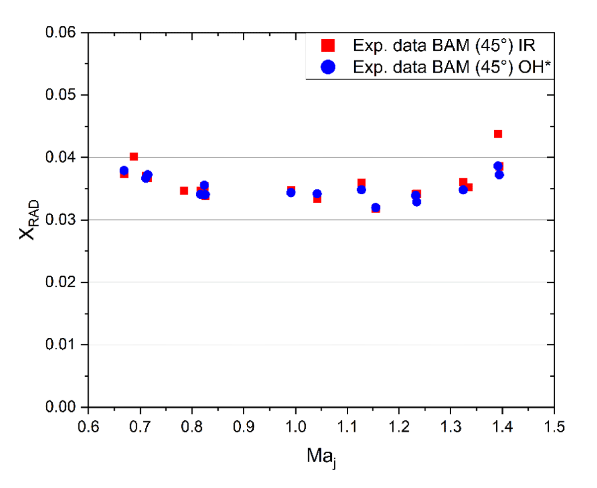
Figure 8
Experimental determined radiant heat fraction determined with OH* and IR measurement over the Mach number Maj.
In Figure 9a, two models are compared against the experimentally determined values for inclined jet flames with IR and OH* cameras. The models are those of Panda and Hecht (2017), and Ekoto et al. (2012). As the measurement principle of the IR camera and the OH* camera differ significantly, adequate models for each type of dataset have to be chosen. As explained earlier, the OH* data describe the pure combustion/reaction zone, while the IR data also include hot flue gases, which represent different physico-chemical processes. The model of Panda and Hecht is based on the residence time as representing the time a molecule is present in the reaction zone, within which it can contribute to the radiation of the flame. This approach was chosen for comparison with the OH* data as these only quantify the reaction zone, in concordance with the model assumptions. The model of Ekoto et al. was chosen as an approach that is not explicitly restricted to the reaction zone and therefore seems suitable for comparison with the IR measurements.
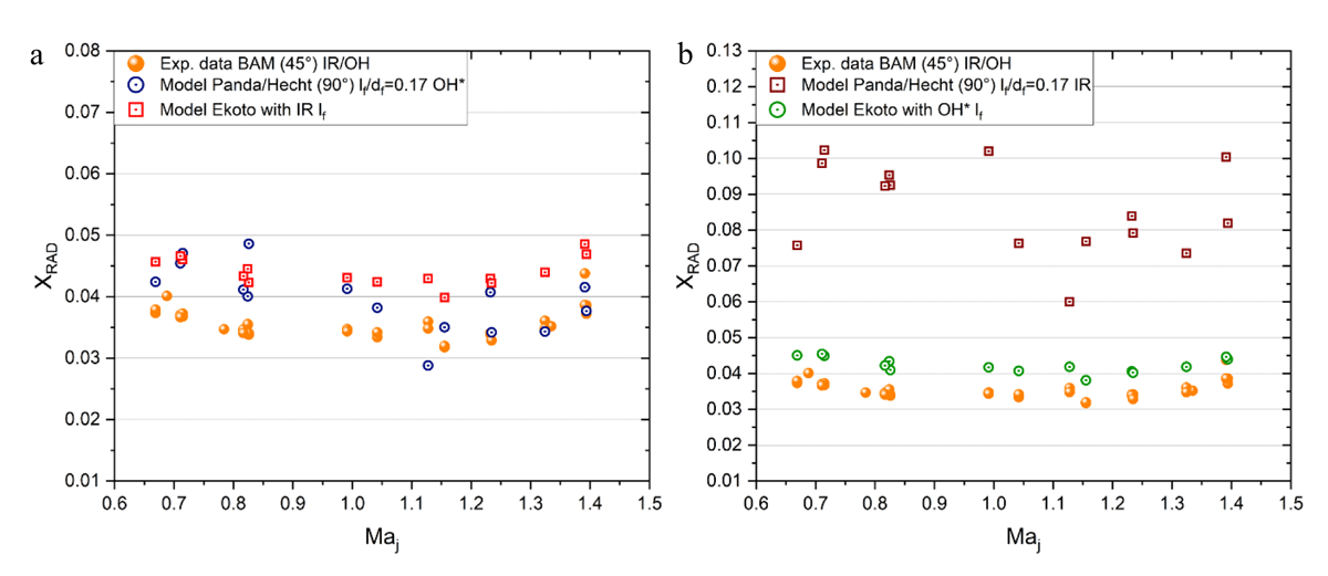
Figure 9
Comparison between experimental determined radiant heat fractions to model of Panda and Hecht using OH* and Ekoto using IR data (a) and Panda and Hecht using IR and Ekoto using OH* (b). The data is plotted against the Mach number Maj.
The model of Panda and Hecht uses the approach of the residence time to calculate the radiant heat fraction according to Eq. (3):
Here, ap is the Planck-mean absorption coefficient (which is 0.23 for hydrogen, see Molina, Schefer and Houf, 2007) and Tad the adiabatic flame temperature. The residence time can be calculated according to Eq. (4):
This approach was developed by Turns and Myhr (1991), who investigated the radiant heat fraction in dependency of the residence time of combustion reactants in a jet flame. The approach takes into account the absorptance of the reactants, flame geometry, combustion properties (temperature, stoichiometry) and fluid mechanic outlet conditions (density, outlet velocity, release diameter). Further investigations and development of this approach were performed by Molina, Schefer and Houf (2007), who expanded this model with flame geometry parameters (constant ratio of flame geometry df/lf). Based on this, Panda and Hecht extended this approach, even for hydrogen jet flames of releases at lower temperatures, using the fixed ratio of flame diameter to flame length stated by Schefer et al. (2006) for vertical jet flames of df/lf = 0.17.
In the model of Ekoto et al. (2012) the radiant heat fraction is modeled using a non-dimensional radiant power factor C*. This radiant factor C* is based on the model of Sivathanu and Gore (1993). As an extension of the approach of Sivathanu and Gore, the multi-source approach of Hankinson and Lowesmith (2012), which includes a weighting of the radiant power to the multi series of point sources (N = 80), is part of the model of Ekoto et al. Except for the flame length (for the even repartition of the multi series of point sources) and the spatial position of the flame centerline, no additional information on the flame shape is required in the model of Ekoto et al. The radiant heat fraction is calculated using the dimensionless radiation factor C* and the distances between the bolometers and the flame Rs via.
C* can be determined with Eqs. (6)–(8):
In Figure 9a, the experimental values for the radiant heat fraction over the Mach number of the expanded jet are compared to the model results. The model of Panda and Hecht was applied to the flame lengths determined by the OH* camera; the model of Ekoto et al. used the flame lengths determined by the IR camera, according to the respective model assumptions as described earlier. Both models show a very good accuracy in predicting the radiant heat fraction compared to the experimental data.
As illustrated in Figure 9b, the performance of each model is demonstrated when applied to values that deviate from the model’s assumptions. In this figure, the experimental values of xRAD over Maj are compared against the model of Panda and Hecht using the IR flame length and the model of Ekoto et al. using the OH* flame length. The model of Panda and Hecht shows a poorer performance than in Figure 9b, now overpredicting the radiant heat fraction. This effect was to be expected since the model formulation is strongly dependent of the length of the reaction zone. The IR recordings exhibit significantly longer flame lengths compared to the OH* recordings (cf. Figure 4), as they include both the reaction zone and the surrounding hot flue gases. Consequently, the residence time predicted by the Panda and Hecht model is overestimated, resulting in a larger value for the radiant heat fraction.
When looking at the values of the model of Ekoto et al. it is very interesting to see that the prediction accuracy is comparable to that in Figure 9a. The reason for this is that the model of Ekoto et al. does not differentiate between the zones in a flame but only considers the flame length (IR or OH*) and the corresponding non-dimensional radiant power C* (IR or OH*) to distribute evenly the combustion energy along the flame. In addition, the model of Ekoto et al. is not based on values that are specific for a certain region of the flame as is the case for the residence time of Panda and Hecht. The model is therefore much less sensitive to the type of detection technology.
4. Conclusion
Inclined jet flame experiments of hydrogen using IR and OH* measurement technique were conducted and compared with existing models. The flame lengths estimated by analyzing the OH* data are considerably shorter than the ones estimated from the IR measurements. The reason for this is that IR measurements cover the entire radiating area, which consists of preheated fuel, the combustion zone and hot flue gases, whereas OH* measurements cover only the combustion zone. These different geometric data on the flame result in significantly different SEPs with the OH* values exceeding the IR values by a factor of 5–6. The calculation of the radiant heat fraction leads to nearly the same results despite the two fundamentally different measurement approaches. The differences in flame length and SEP compensate in such a way that nearly equal radiant heat fraction values are found, in the range of approximately 0.031–0.043.
The comparison with two radiation models showed a good concordance with the experimental data if the application limits of the models are respected. The model of Panda and Hecht, focused on processes in the combustion zone, can only be used with the OH* results (showing only the combustion zone) and shows large deviations when used outside the application limits with, e.g. the IR results (showing the combustion zone and all other hot gases). The model of Ekoto et al., which is based on more general considerations and therefore independent of specific flame zones, shows a good performance using the OH* and IR results.
Acknowledgements
This work is part of the competence center H2Safety@bam in the field of process and plant safety at the Bundesanstalt für Materialforschung und -prüfung (BAM). The authors would like to thank all partners of the project for discussions and exchange of ideas. The authors are thankful to Prof. C. O. Paschereit for enabling the use of a camera equipped with OH* filter at the BAM test site.
Competing Interests
Christopher Bernardy and Abdel Karim Habib reports a relationship with Bundesanstalt fuer Materialforschung und -pruefung that includes: employment. Philipp zur Nedden, Jakob von Saldern, Jan Beuth and Alessandro Orchini reports a relationship with Technical University of Berlin that includes: employment.
Author Contributions
Conceptualization: K.H., A.O.; Data curation: C.B., K.H. P.M.z.N.; Formal analysis: C.B., K.H., Investigation: C.B., K.H., P.M.z.N, J.G.R.v.S., J.P.B; A.O.; Resources: K.H., C.B., P.M.z.N., A.O.; Methodology: C.B., K.H., P.M.z.N., J.G.R.v.S., J.P.B; A.O.; Project administration: K.H., C.B.; Software: C.B., K.H., P.M.z.N.; Validation: C.B., K.H.; Supervision: K.H., A.O.; Visualization: C.B.; Writing – original draft: C.B.; Writing – review and editing: C.B., K.H., P.M.z.N, J.G.R.v.S., J.P.B; A.O.