
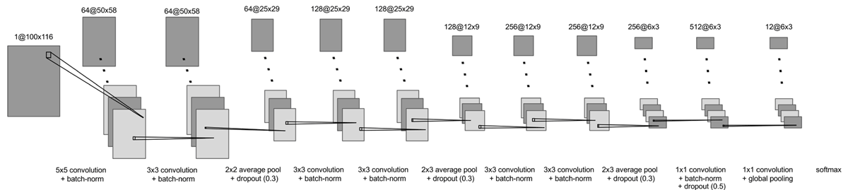
Figure 1
CNN architecture of the instrument classifier. Input: channels@mel bands × windows.
Table 1
Notation of variables.
| Variable | Meaning |
|---|---|
| x | Original signal |
| y | Ground-truth label |
| X | Time-frequency representation of x |
| δ | Adversarial perturbation |
| Adversarial example | |
| t | Target class/prediction |
| f | System (e.g., instrument classifier) |
| Lsys | System-specific loss function (e.g., cross-entropy loss) |
| ∇x | Gradient w.r.t. x |
| η | Multiplication factor for updates |
| ep | Current iteration |
| δep | Perturbation during iteration ep |
| α | Weight factor for adversarial objective |
| ɛ | Clipping factor for updates |
Table 2
Comparison of the adversarial attacks on our instrument classifier. Results are chosen based on largest SNR with at least 150 (lines 4 to 7) and 180 (lines 8 to 11) successfully found adversarial examples out of 200. Depicted are averages or the median over samples; for the PGD-Attack, C&W and Multi-Scale C&W additionally average and standard deviation* of results over five runs are stated. Line 3 contains a baseline with random white-noise instead of adversarial perturbations.
| Samples Required | Data Origin | # Samples | Accuracy | SNR | Iterations |
|---|---|---|---|---|---|
| Clean | 200 | 0.835 | – | – | |
| White-noise | 200 | 0.785 ± 0.000* | 42.71 ± 0.00* | – | |
| min.150 | FGSM | 153 | 0.250 | –7.74 | 1.0 |
| PGD-Attack | 151.8 ± 0.7* | 0.171 ± 0.004* | 40.13 ± 0.05* | 15.8 ± 0.4* | |
| C&W | 153.2 ± 2.6* | 0.201 ± 0.016* | 44.23 ± 0.37* | 51.4 ± 2.7* | |
| C&Wmulti_scale | 163.6 ± 3.0* | 0.167 ± 0.012 * | 43.82 ± 0.09* | 71.6 ± 5.4* | |
| min.180 | FGSM | 179 | 0.130 | –24.83 | 1.0 |
| PGD-Attack | 190.8 ± 1.2* | 0.026 ± 0.004* | 16.47 ± 0.10* | 2.0 ± 0.0* | |
| C&W | 180.2 ± 2.3* | 0.094 ± 0.010* | 42.98 ± 0.18* | 66.1 ± 3.7* | |
| C&Wmulti_scale | 196.4 ± 1.0* | 0.024 ± 0.004* | 39.49 ± 0.17* | 22.6 ± 1.0* |
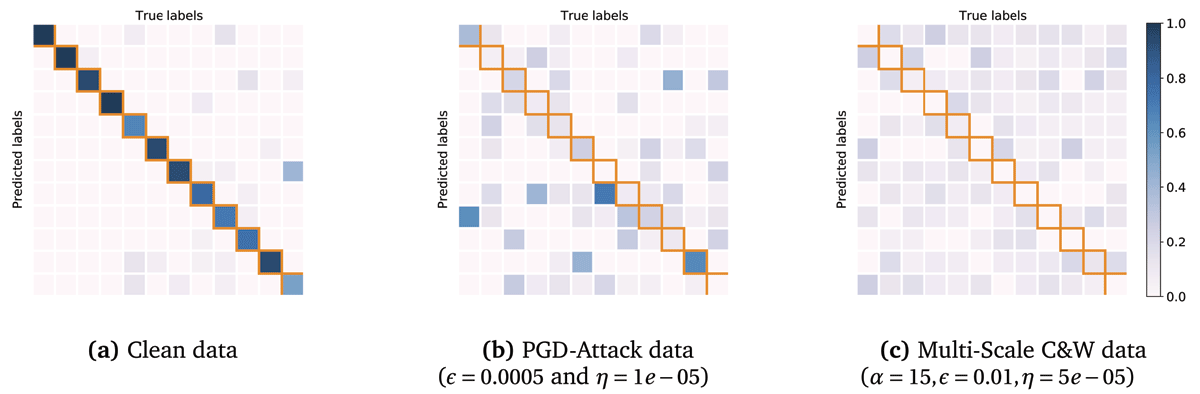
Figure 2
Confusion matrices computed on validation data, showing correct predictions in the diagonal, confusions off-diagonal. For samples without adversarial counterpart, original audio is used. Columns are ground-truth labels and rows predictions; columns are normalised to sum to 1. Order of labels (left to right and top to bottom): Accordion, Acoustic guitar, Bass drum, Bass guitar, Electric guitar, Female singing, Glockenspiel, Gong, Harmonica, Hi-hat, Male singing, and Marimba/xylophone.
Table 3
Results of adversarial C&W attack on music recommendation system for varying hub-sizes. SNR and k-occurrence expressed by mean ± standard deviation over all adversarial examples, the number of which is indicated by the number in column 3.
| Hub-size | # Hubs (before) | # Hubs (after) | # Non-hubs (after) | SNR | k-occurrence |
|---|---|---|---|---|---|
| 25 | 644 (4.1%) | 6,381 (40.5%) | 8,725 (55.4%) | 39.12 ± 5.50 | 48.50 ± 31.42 |
| 50 | 203 (1.3%) | 4,313 (27.4%) | 11,234 (71.3%) | 38.82 ± 5.02 | 85.34 ± 43.77 |
| 75 | 83 (0.5%) | 3,080 (19.6%) | 12,587 (79.9%) | 38.83 ± 4.58 | 119.55 ± 56.05 |
| 100 | 32 (0.2%) | 2,357 (15.0%) | 13,361 (84.8%) | 38.69 ± 4.33 | 153.05 ± 64.89 |
| 125 | 14 (0.1%) | 2,244 (14.2%) | 13,492 (85.7%) | 38.46 ± 4.18 | 183.03 ± 71.89 |
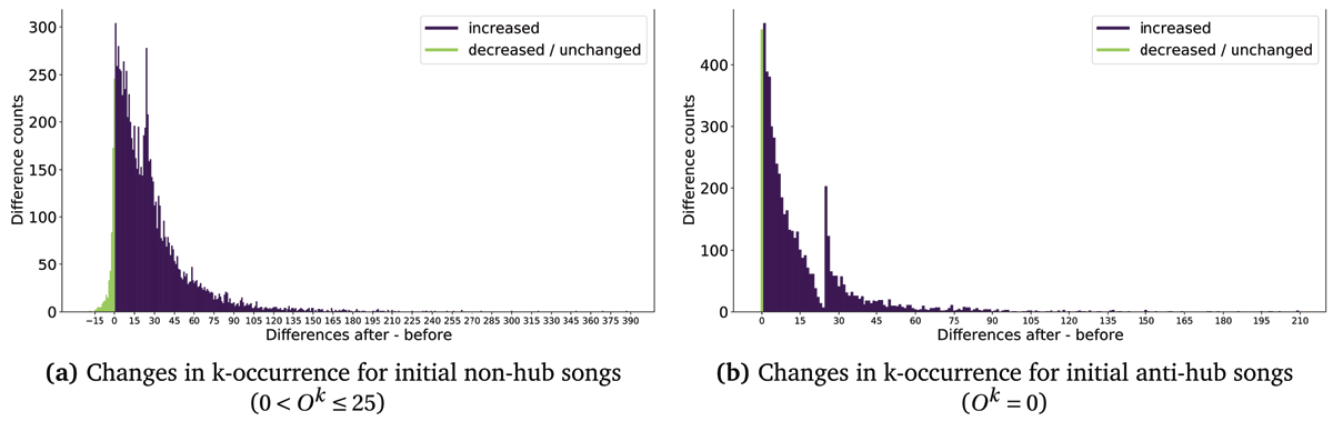
Figure 3
Histogram of changes in k-occurrence before and after the C&W attack on the music recommendation system for a hub-size of 25. Changes larger than zero denote an increase of the k-occurrence after an attack.