
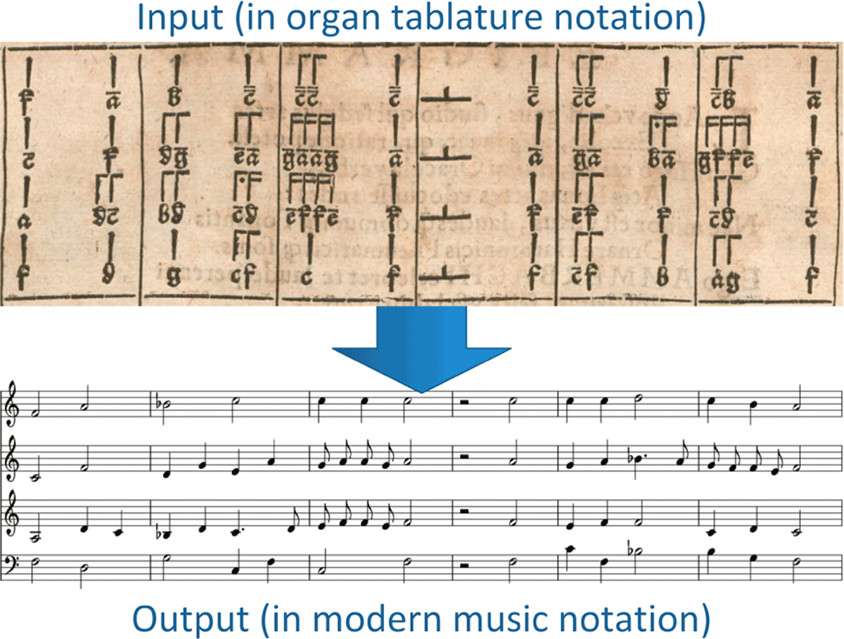
Figure 1
Transcription of a tablature row into modern music notation. The transcribed row consists of four tablature staves that are converted into a four-part score in modern notation.
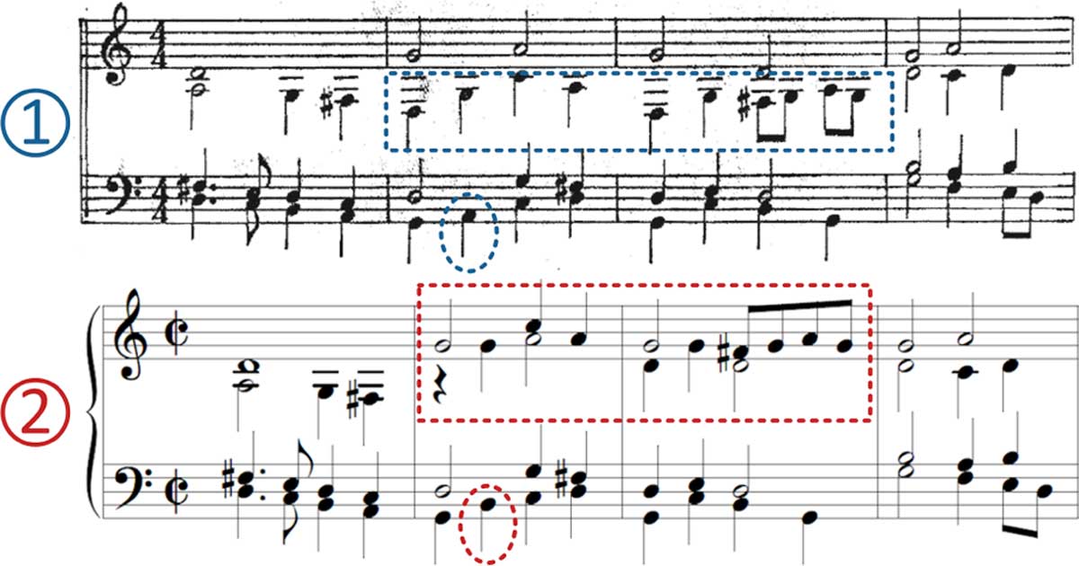
Figure 2
Deviations in transcriptions of Ammerbach’s “Orgel oder Instrument Tabulaturbuch” by (1) Becker (1963) and (2) Müller-Schmidt (2017).
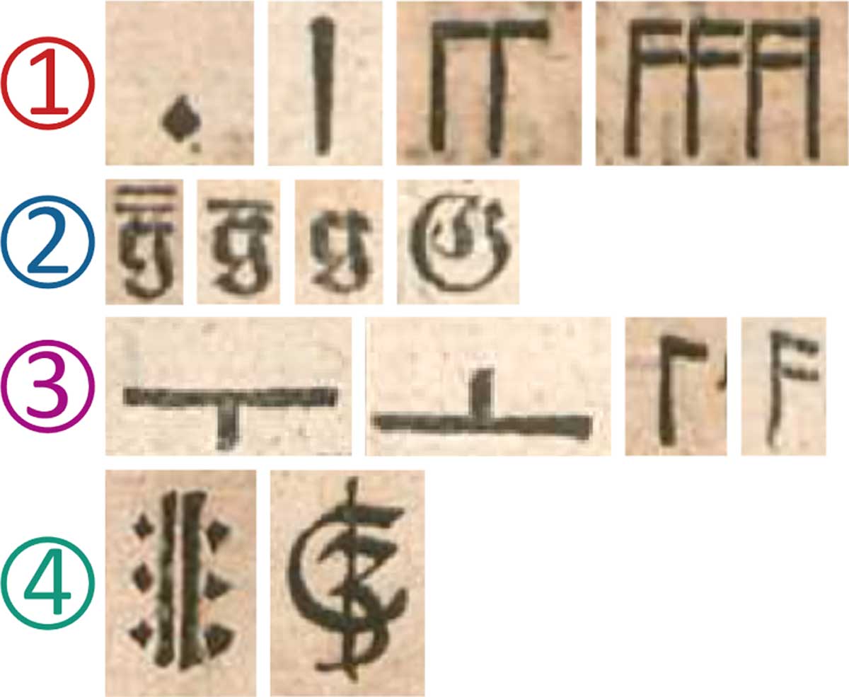
Figure 3
Examples of the different types of organ tablature symbols taken from Ammerbach (1583): (1) Note duration symbols; (2) Note pitch symbols; (3) Pause signs; (4) Special characters.
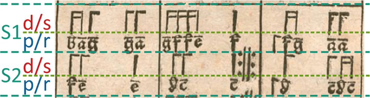
Figure 4
The layout of printed tablature characters using the example of Ammerbach (1583). Each staff (S1, S2) inside the row consists of two lines (duration/special (d/s) and pitch/rest (p/r) line) in which the tablature characters are arranged.

Figure 5
Segmentation of the input image. The input image is split into separate images for each row on the displayed horizontal dividing lines. Afterwards, the results are split into images for each staff using the estimated voice positions.
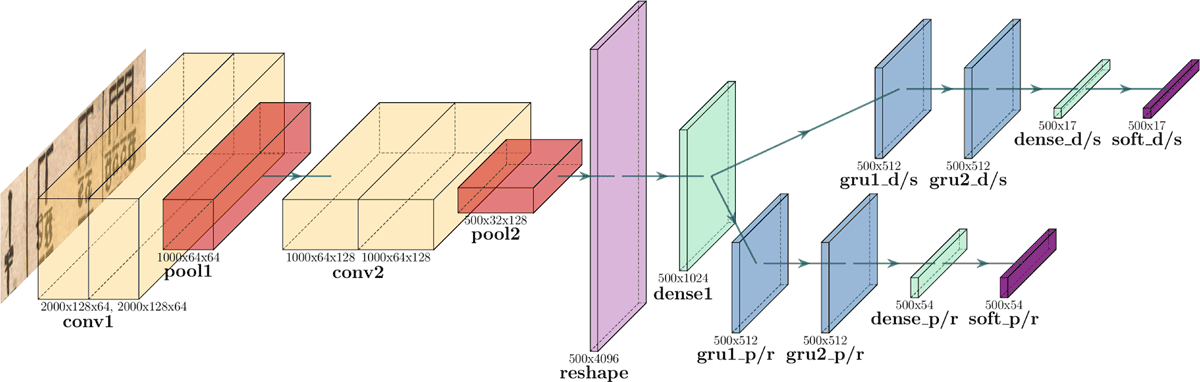
Figure 6
Architecture of the CSP tablature recognition network. The different layer types are color-coded and the size is indicated below each layer. This image was generated with PlotNeuralNet (Iqbal, 2018).
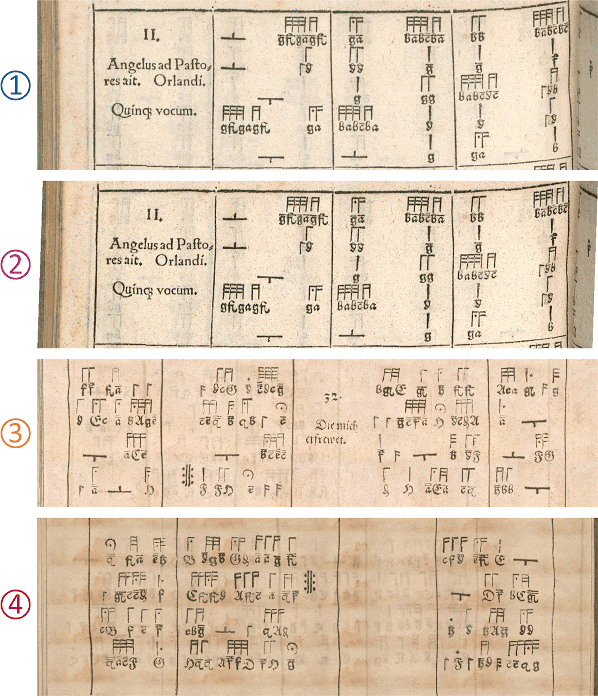
Figure 7
Comparison of (1) a real tablature row from Ammerbach’s tablature books; (2) an augmented version of the same tablature row; (3,4) two tablature rows artificially created by the data generator.
Table 1
The data set, consisting of training, evaluation, and test sets. The values indicate the number of images taken from each source. The numbers in parentheses indicate the factor by which this number has been enlarged by data augmentation.
| Subset | Staves taken from “Orgel oder Instrument Tabulaturbuch” | Staves taken from “Ein new künstlich Tabulaturbuch” | Generated Staves | Sum |
|---|---|---|---|---|
| trainSetL | 500 (*100) | 500 (*100) | 140,000 (*5) | 800,000 |
| trainSetS | 500 (*100) | 500 (*100) | 20,000 (*5) | 200,000 |
| valSet | 200 (*25) | 200 (*25) | 8,000 (*5) | 50,000 |
| testSet | 500 | 500 | 0 | 1,000 |
Table 2
Comparison of the CSP network with two partial networks, one for each path. The table shows the metrics evaluated on the test data set, the number of floating point operations (FLOPs), and the training time required for 40 epochs.
| Network | Characters | Accuracy | Edit Distance | Computation Time | |||||
|---|---|---|---|---|---|---|---|---|---|
| Top-10 | Top-5 | Top-1 | Bar | Staff | Char | FLOPs | Training | ||
| CSP | Duration/Special | 0.994 | 0.992 | 0.970 | 0.989 | 0.070 | 0.00162 | 27,925,688 | 47h34m |
| Pitch/Rest | 0.944 | 0.943 | 0.876 | 0.971 | 0.320 | 0.00515 | |||
| Partial 1 | Duration/Special | 0.991 | 0.990 | 0.963 | 0.988 | 0.086 | 0.00192 | 18,377,884 | 28h12m |
| Partial 2 | Pitch/Rest | 0.963 | 0.960 | 0.896 | 0.972 | 0.250 | 0.00423 | 18,453,660 | 32h33m |
Table 3
Comparison of the CSP network with three simpler variations of the network. The table shows the differences in the network configurations, the metrics evaluated on the test set, as well as the number of FLOPs for each network.
| Network | Configuration | Characters | Accuracy | Edit Distance | FLOPs | |||
|---|---|---|---|---|---|---|---|---|
| CNNs | GRUs | Top-1 | Bar | Staff | Char | |||
| Full CSP | 2 blocks | 2 bidir. | Duration/Special | 0.970 | 0.989 | 0.070 | 0.00162 | 27,925,688 |
| 2 bidir. | Pitch/Rest | 0.876 | 0.971 | 0.320 | 0.00515 | |||
| 1 CNN | 1 block | 2 bidir. | Duration/Special | 0.954 | 0.989 | 0.095 | 0.00218 | 27,483,320 |
| 2 bidir. | Pitch/Rest | 0.840 | 0.958 | 0.501 | 0.00835 | |||
| unidir. GRUs | 2 blocks | 2 unidir. | Duration/Special | 0.962 | 0.988 | 0.079 | 0.00190 | 18,415,780 |
| 2 unidir. | Pitch/Rest | 0.835 | 0.960 | 0.412 | 0.00690 | |||
| 1 GRU | 2 blocks | 1 bidir. | Duration/Special | 0.950 | 0.984 | 0.098 | 0.00207 | 21,634,212 |
| 1 bidir. | Pitch/Rest | 0.818 | 0.949 | 0.516 | 0.00859 | |||
Table 4
Comparison of training the CSP network with different data sets. The table shows the differences in the number of real and generated tablature images (as well as the factor by which this amount was increased by augmentation) for each training set and the metrics evaluated on the test data.
| Train Data | Number of Tablature Staves | Characters | Accuracy | Edit Distance | ||||
|---|---|---|---|---|---|---|---|---|
| Real | Generated | Sum | Top-1 | Bar | Staff | Char | ||
| noAug | 1000 | 0 | 1000 | Duration/Special | 0.844 | 0.952 | 0.348 | 0.00746 |
| Pitch/Rest | 0.641 | 0.895 | 1.270 | 0.02258 | ||||
| Aug | 1000 (*100) | 0 | 100,000 | Duration/Special | 0.966 | 0.995 | 0.063 | 0.00134 |
| Pitch/Rest | 0.851 | 0.967 | 0.394 | 0.00645 | ||||
| Aug1Gen1 | 1000 (*100) | 20,000 (*5) | 200,000 | Duration/Special | 0.970 | 0.993 | 0.055 | 0.00120 |
| Pitch/Rest | 0.875 | 0.972 | 0.286 | 0.00455 | ||||
| Aug1Gen2 | 1000 (*100) | 40,000 (*5) | 300,000 | Duration/Special | 0.967 | 0.990 | 0.068 | 0.00143 |
| Pitch/Rest | 0.873 | 0.970 | 0.307 | 0.00510 | ||||
| Aug2Gen2 | 1000 (*200) | 40,000 (*5) | 400,000 | Duration/Special | 0.971 | 0.990 | 0.059 | 0.00128 |
| Pitch/Rest | 0.870 | 0.972 | 0.292 | 0.00475 | ||||
| PtAug | 100 (*100) | 0 | 10,000 | Duration/Special | 0.725 | 0.919 | 0.782 | 0.01608 |
| Pitch/Rest | 0.527 | 0.849 | 2.005 | 0.03460 | ||||
| PtAugGen | 100 (*100) | 50,000 (*5) | 260,000 | Duration/Special | 0.871 | 0.952 | 0.266 | 0.00583 |
| Pitch/Rest | 0.709 | 0.906 | 0.864 | 0.01539 | ||||
Table 5
Evaluation of the CSP network trained on the trainSetS data set. The table shows the metrics calculated on the test data set.
| Characters | Accuracy | Edit Distance | ||||
|---|---|---|---|---|---|---|
| Top-10 | Top-5 | Top-1 | Bar | Staff | Char | |
| Duration/Special | 0.996 | 0.996 | 0.970 | 0.993 | 0.055 | 0.00120 |
| Pitch/Rest | 0.951 | 0.947 | 0.875 | 0.972 | 0.286 | 0.00455 |
Table 6
The errors that occurred during the analysis, categorized into groups with the corresponding number of cases.
| Duration/Special Errors | Pitch/Rest Errors | ||
|---|---|---|---|
| Category | Count | Category | Count |
| Missed Symbol | 21 | Missed Symbol | 47 |
| Added Symbol | 4 | Added Symbol | 17 |
| Wrong Symbol | 10 | Wrong Symbol | 74 |
| Wrong Octave | 85 | ||
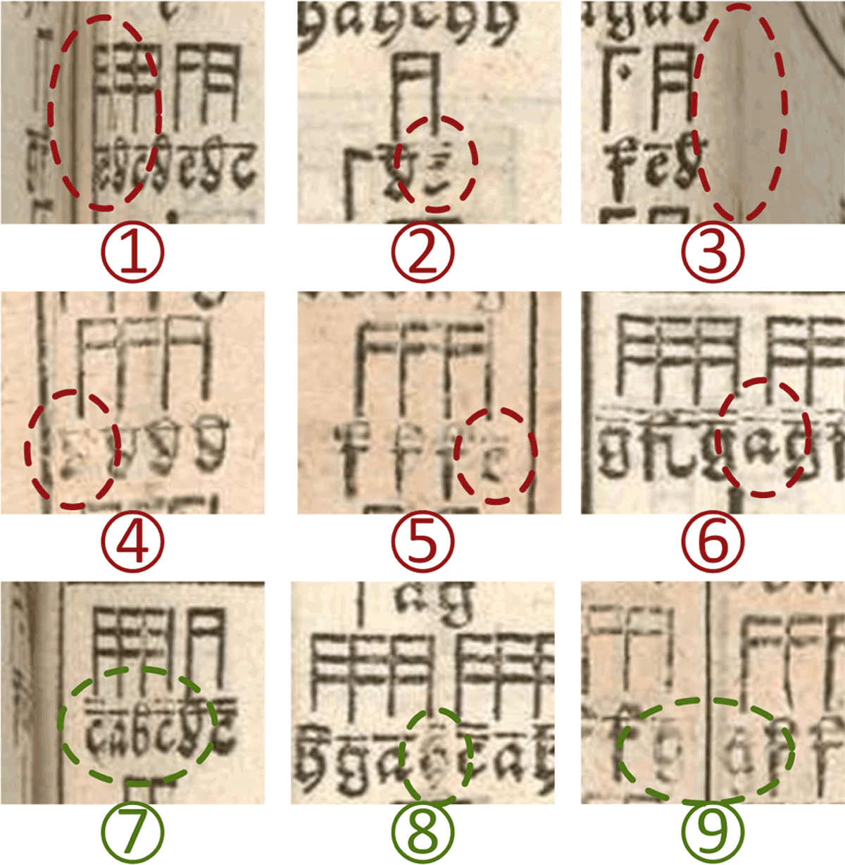
Figure 8
Examples of areas in the test data that are difficult to recognize. In images 1–6, an analysis error occurred in the marked areas, while in images 7–9, even in the circled areas, the poorly readable characters were correctly recognized.