
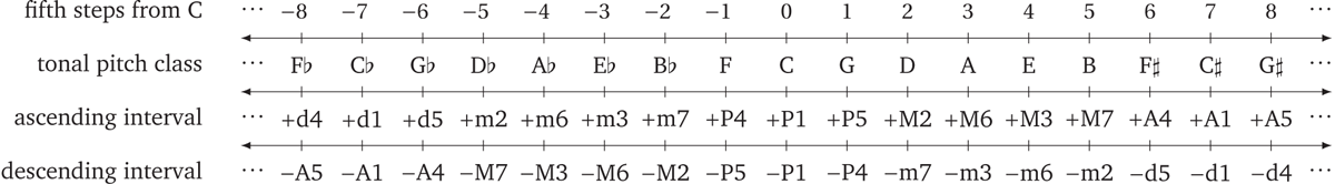
Figure 1
Tonal space ℑ and interval space ℐ on line of fifths: tonal pitch-classes and tonal pitch-class intervals along with their integer representation in terms of the number of steps along the line of fifths (using C as a reference tone).
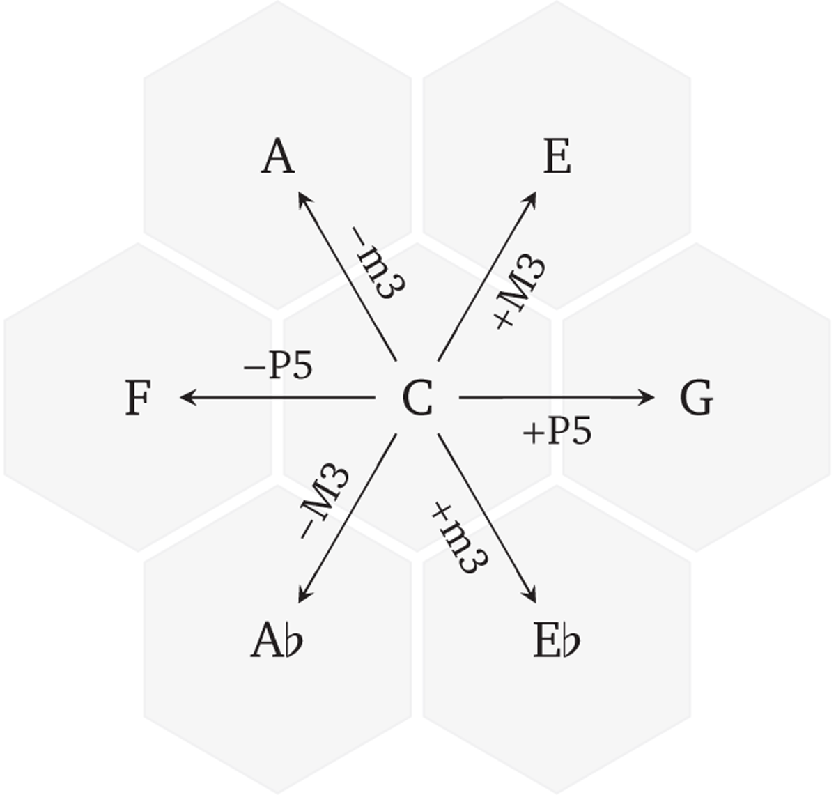
Figure 2
Primary intervals with respect to C.
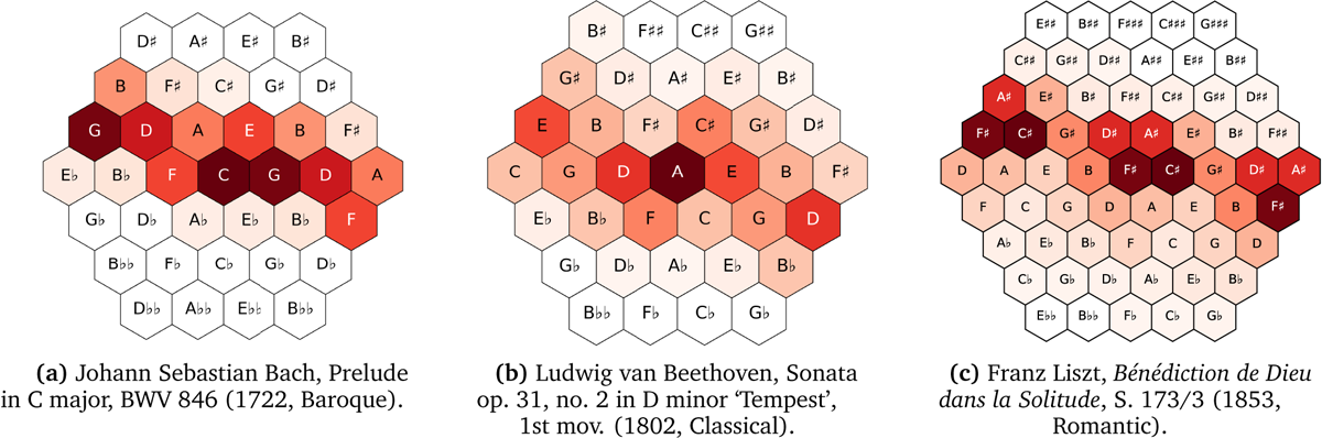
Figure 3
Tonal pitch-class distributions plotted as heatmaps on the Tonnetz (darker colors correspond to higher probabilities). The plots were generated with the Python library pitchplots (Moss et al., 2019).
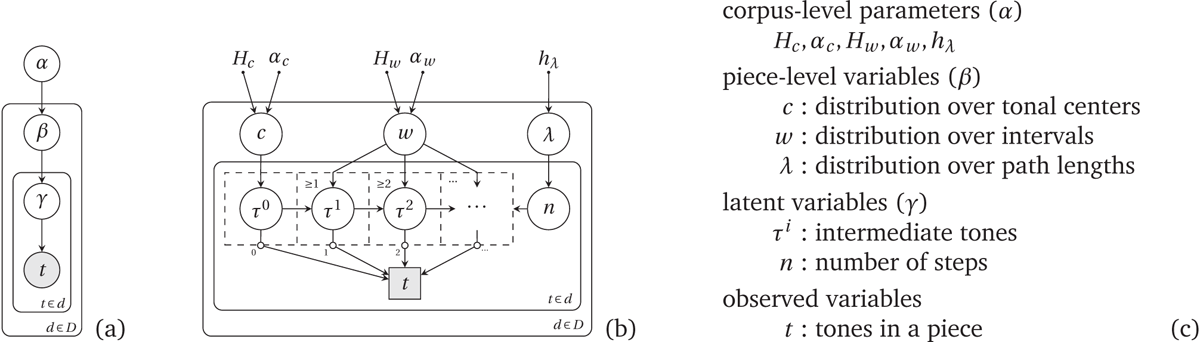
Figure 4
(a) General structure of a topic model. (b) The Tonal Diffusion Model. We use an extended gate notation (Minka and Winn, 2009): random variables in dashed boxes and edges connected via a gate (empty circles) exist only if the random variable connected to the border (n in this case) fulfills the condition in the top-left corner or next to the gate, respectively. (c) Overview of the variables and parameters, see Section 4.1 for more details.
Algorithm 1
Computing the marginal likelihood p(t|c,w,λ) by explicitly marginalizing out the latent variables γ≡ (τ0,…, τn,n). In practice, the infinite loop over n is terminated by summing over p(n|λ) and stopping when this cumulative probability approaches 1 (with tolerance 10–5).
| Input: Output: c,w,λ | |||
| Output: p(t|c,w,λ) | |||
| 1: | u ← 0 | # initialize output distribution | |
| 2: | v ← p(τ0|c) | # initialize intermediate distribution | |
| 3: | M ← p(τ′|τ,w) | # initialize transition matrix | |
| 4: | for n ∈ {0,1,…} do | ||
| 5: | u ← u + p(n|λ) · v | # update, marginalizing out n | |
| 6: | v ← Mv | # transition, marginalizing out τi | |
| 7: | end for | ||
| 8: | return u | ||
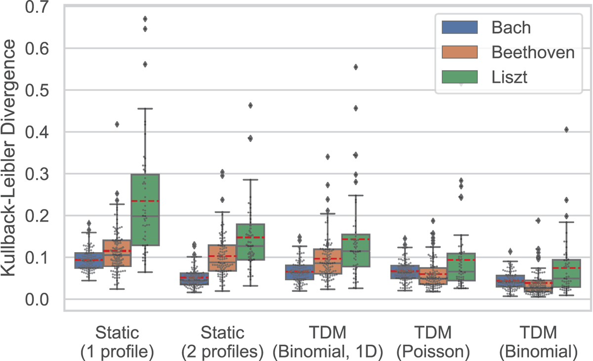
Figure 5
Comparison of model performance for composers from different historical epochs: Bach (Baroque), Beethoven (Classical), Liszt (Romantic). The box plots indicate quartiles (25%, 50%, 75%), whiskers extend 1.5 times the interquartile range (IQR). The mean is indicated as a dashed red line. Single pieces are shown as black dots in a swarm plot, outliers as larger diamonds.
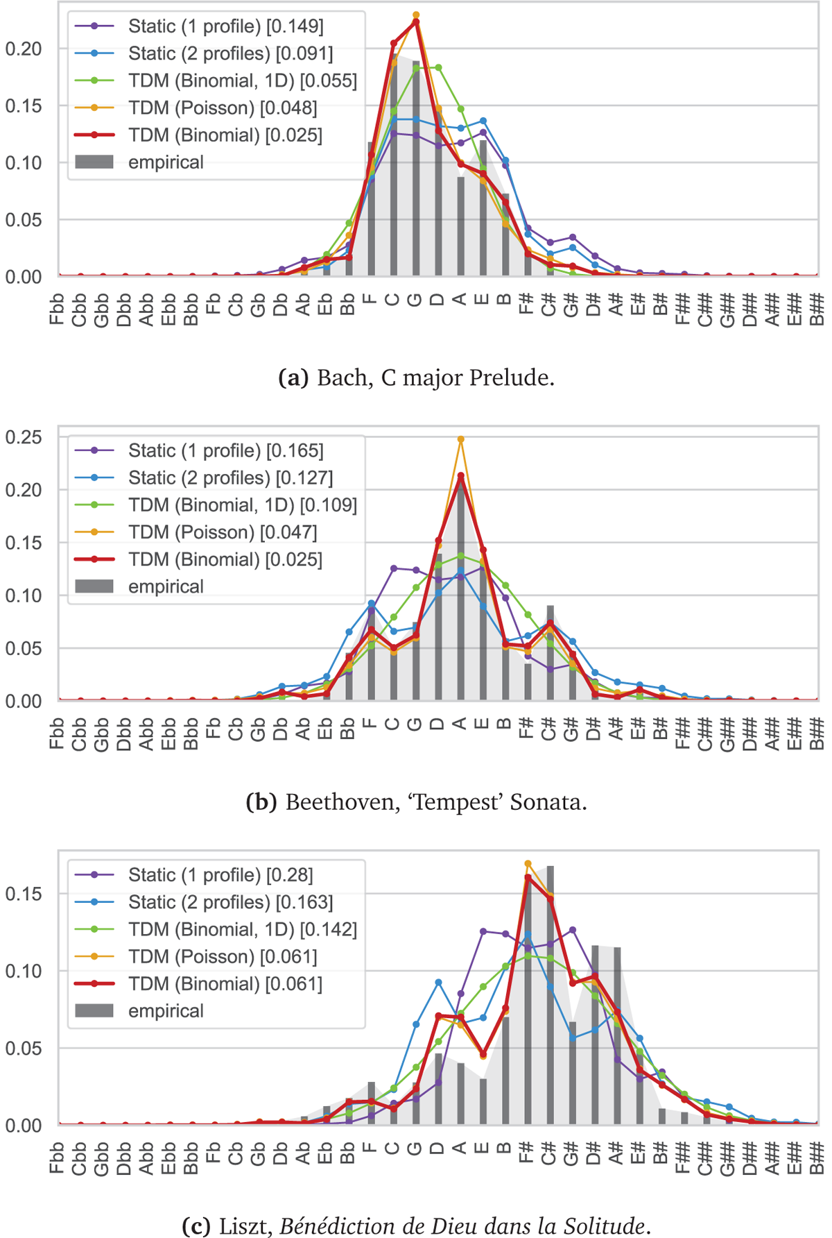
Figure 6
Comparison of the empirical PCD (gray bars with shaded background) with different models (colored plots). The corresponding Kullback-Leibler divergence is indicated in square brackets after the model.
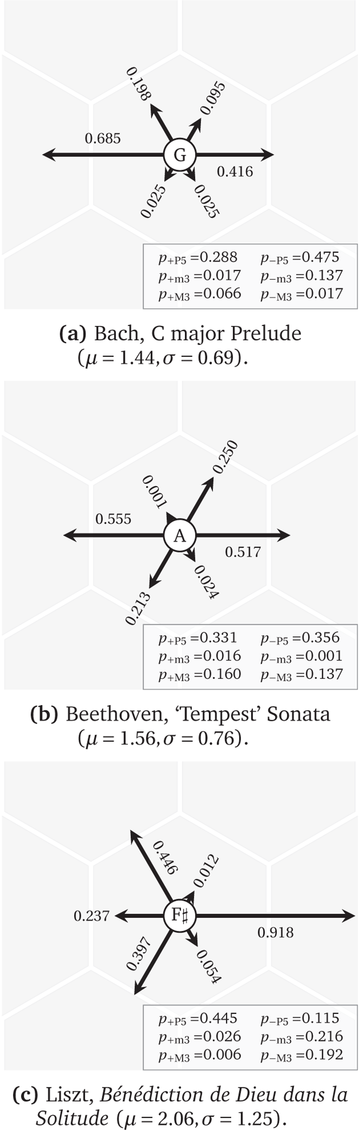
Figure 7
Optimal parameters for the TDM (Binomial) model (see text for details).