
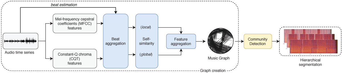
Figure 1
Schematic overview of MSCOM with all the main steps of its workflow.
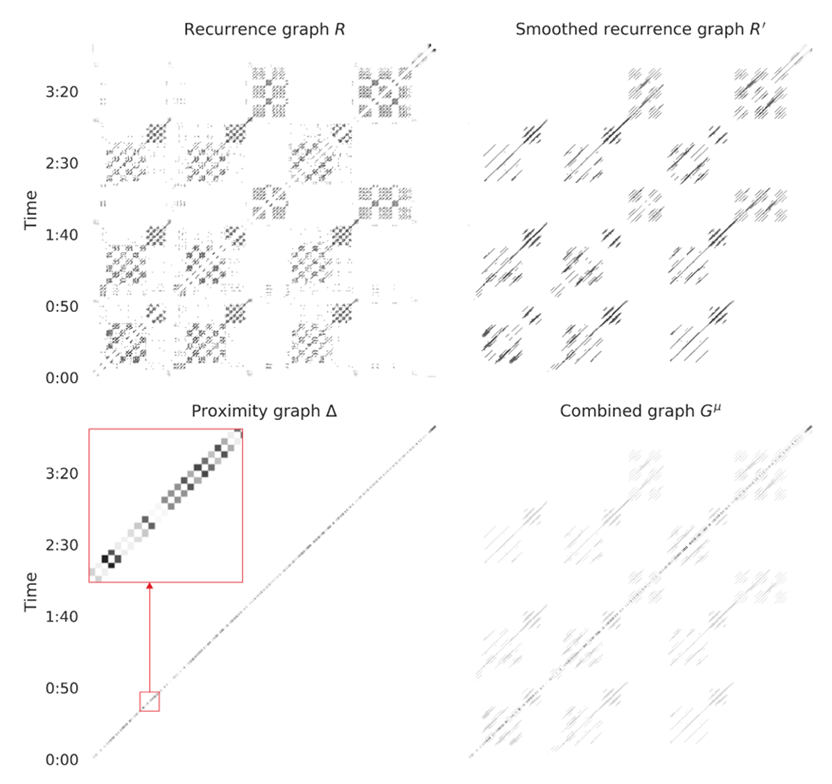
Figure 2
The main steps detailed in Section 3.1 for the creation of the music graph for the track “SALAMI 676”. The recurrence graph R computed on the chroma features and its smoothed version R′ to enhance diagonal stripes are illustrated in the top quadrants. The bottom-left plot represents the proximity graph Δ with a zoomed area highlighting its upper and lower off-diagonals that ensure the linkage of nodes corresponding to temporally consecutive feature vectors. The graph Gµ in the last quadrant is a weighted sum of R′ and Δ as outlined in Equation 4.
Algorithm 1
Hierarchical community detection
| Given the N × N adjacency matrix W of a graph | |
| Given Δr, a fixed step increment for r | |
| Let W[S] be the square sub-matrix obtained by selecting the rows and columns of W with index in S | |
| 1: l ←1 | |
| 2: | |
| 3: W ← W + rI | |
| 4: | ▷ all node indices in |
| 5: While |Cl|< N do | |
| 6: l ←l+ | 1▷current level |
| 7: Cl ← {} | |
| 8: | |
| 9: | |
| optimal partition of | |
| 10: | |
| 11: end for | |
| 12: r ← r + Δr | |
| 13: W ← W + rI | |
| 14: end while | |
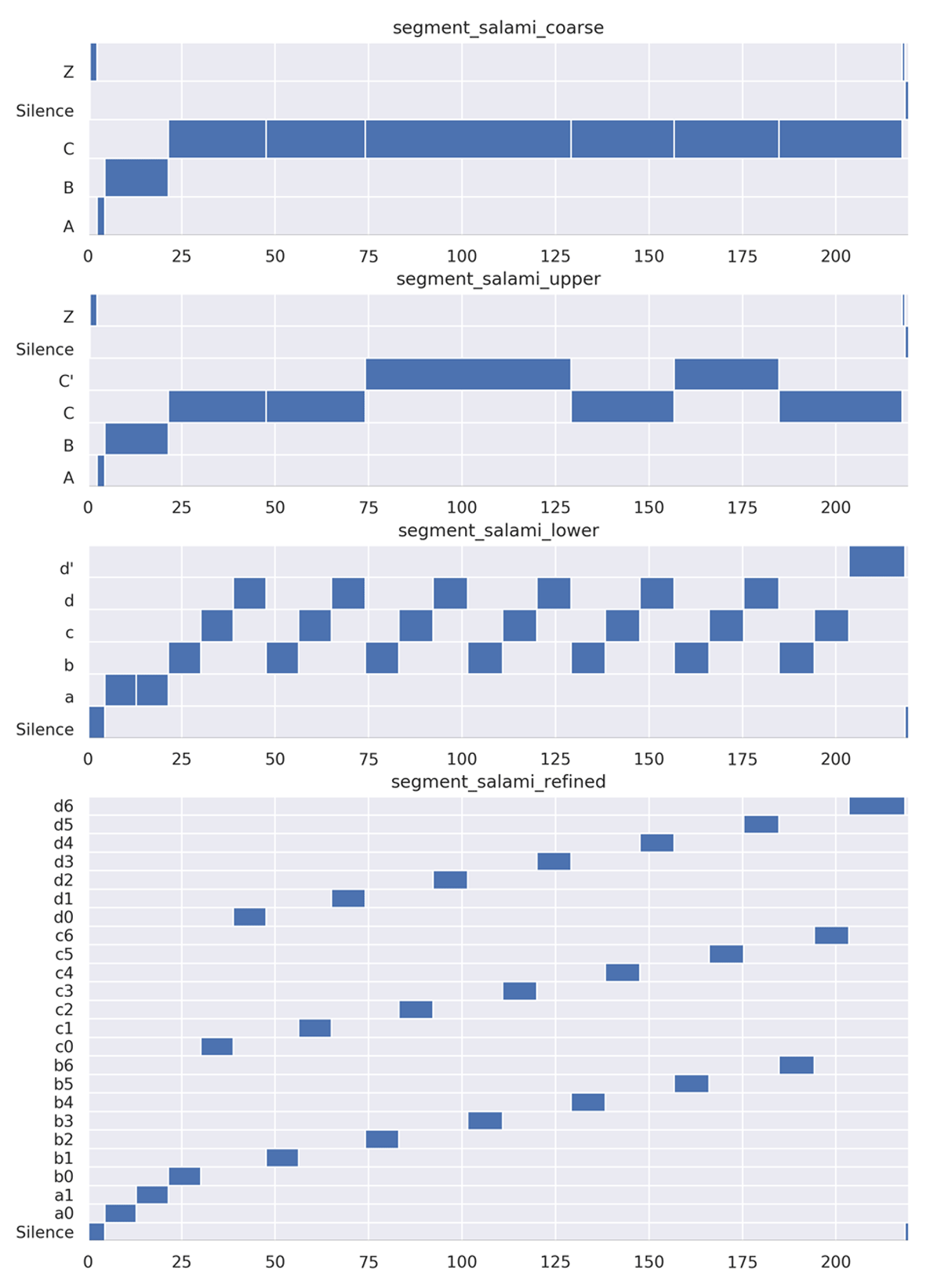
Figure 3
Hierachical expansion of the first human annotation of SALAMI 1094. The two segmentation levels denoted with the upper and lower tags define the original hierarchy, whereas the coarse and the refined levels are obtained by contracting the upper level and refining the lower level respectively.
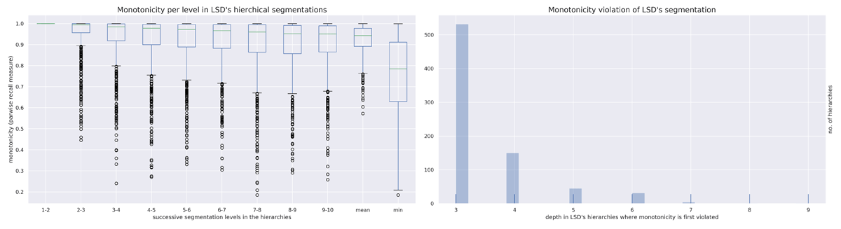
Figure 4
Analysis of monotonicity in LSD’s hierarchical segmentations. Left: distribution of monotonicity for each couple of successive levels in the hierarchies estimated by LSD. Right: distribution of the level (or depth) in LSD’s hierarchies at which maximum monotonicity is no longer preserved.
Table 1
Overview of the segmentation performance - mean and standard deviation of the L-measures - of each algorithm under analysis with respect to the first reference annotation provided for each track in the SALAMI dataset. The evaluation is performed for both the original (left) and the extended (right) reference hierarchies.
| Original reference hierarchies | Extended reference hierarchies | ||||||
| L-measure | L-precision | L-recall | L-measure | L-precision | L-recall | ||
| LSD | 0.462 ± 0.128 | 0.394 ± 0.120 | 0.584 ± 0.150 | 0.480 ± 0.123 | 0.420 ± 0.120 | 0.577 ± 0.143 | |
| LSDM | 0.301 ± 0.179 | 0.377 ± 0.158 | 0.289 ± 0.205 | 0.309 ± 0.179 | 0.402 ± 0.158 | 0.282 ± 0.194 | |
| OLDA | 0.398 ± 0.101 | 0.325 ± 0.098 | 0.536 ± 0.111 | 0.415 ± 0.097 | 0.348 ± 0.098 | 0.531 ± 0.104 | |
| MSCOM | 0.460 ± 0.112 | 0.382 ± 0.102 | 0.600 ± 0.135 | 0.478 ± 0.105 | 0.408 ± 0.098 | 0.593 ± 0.129 | |
| DMSCOM | 0.480 ± 0.111 | 0.403 ± 0.103 | 0.611 ± 0.133 | 0.500 ± 0.104 | 0.430 ± 0.100 | 0.607 ± 0.127 | |
Table 2
Summary of the Kolmogorov-Smirnov statistical tests used to detect statistically significant differences between the algorithms’ performance on each evaluation metric. For each measure, ‘O’ denotes the evaluation performed on the original reference hierarchies, whereas ‘E’ refers to the extended counterpart. ns: not significant, p > 0.05; * p ≤ 0.05; ** p ≤ 0.01; *** p ≤ 0.001.
| L-measure | L-precision | L-recall | ||||
| O | E | O | E | O | E | |
| MSCOM | ||||||
| LSD | ns | ns | ns | * | ns | ns |
| LSDM | *** | *** | *** | *** | *** | *** |
| OLDA | *** | *** | *** | *** | *** | *** |
| DMSCOM | ||||||
| LSD | *** | *** | *** | *** | * | ** |
| LSDM | *** | *** | *** | *** | *** | *** |
| OLDA | *** | *** | *** | *** | *** | *** |
| MSCOM | ** | ** | *** | *** | ns | ns |
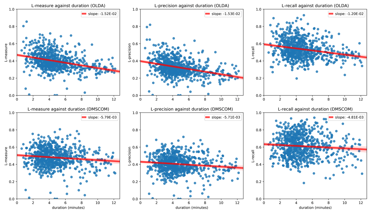
Figure 5
Segmentation performance degradation, in terms of the L measures outlined in Section 4.2, as function of track duration. The first row reports the trend for the evaluation of OLDA, whereas the second one is related to DMSCOM. A regression line is plotted along with the data to facilitate the comparison of the graphs.