
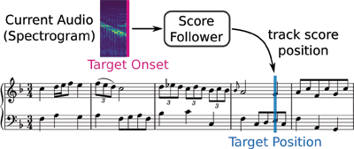
Figure 1
Sketch of score following in sheet music. Given the incoming audio, the score follower has to track the corresponding position in the score (image).
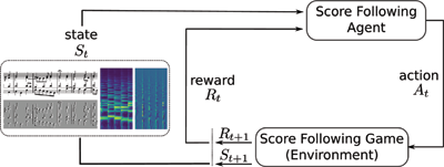
Figure 2
Sketch of the score following MDP. The agent receives the current state of the environment St and a scalar reward signal Rt for the action taken in the previous time step. Based on the current state it has to choose an action (e.g., decide whether to increase, keep or decrease its speed in the score) in order to maximize future reward by correctly following the performance in the score.
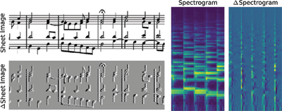
Figure 3
Markov state of the score following MDP: the current sheet sliding window and spectrogram excerpt. To capture the dynamics of the environment we also add the one step differences (Δ) w.r.t. the previous time step (state).
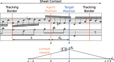
Figure 4
Reward definition in the score following MDP. The reward Rt (range [0, 1]) decays linearly with the agent’s distance dx from the current true score position x.
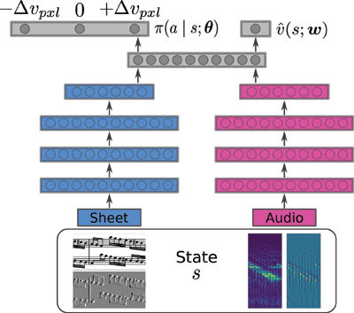
Figure 5
Multi-modal network architecture used for our score following agents. Given state s, the policy network predicts the action selection probability π (a|s;θ) for the allowed actions a ∈ {–Δνpxl, 0, +Δνpxl}. The value network, sharing parameters with the policy network, provides a state-value estimate ̂v(s;w) for the current state.
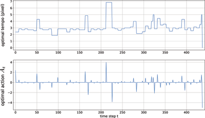
Figure 6
Optimal tempo curve and corresponding optimal actions At for a continuous agent (piece: J. S. Bach, BWV994). The At would be the target values for training an agent with supervised, feed-forward regression.
Table 1
Network architecture used for the Nottingham dataset. Conv (3, stride-1)-16: 3 × 3 convolution, 16 feature maps and stride 1. No zero-padding is applied. We use ELU activation on all layers if not stated otherwise.
| Audio (Spectrogram) 78 × 40 | Sheet-Image 40 × 150 |
|---|---|
| Conv (3, stride-2)-16 | Conv (5, stride-(1, 2))-16 |
| Conv (3, stride-2)-32 | Conv (3, stride-2)-32 |
| Conv (3, stride-2)-32 | Conv (3, stride-2)-32 |
| Conv (3, stride-1)-64 | Conv (3, stride-(1,2))-64 |
| Concatenation + Dense (256) | |
| Dense (256) | Dense (256) |
| Dense (3) – Softmax | Dense (1) – Linear |
Table 2
Network architecture used for MSMD. DO: Dropout; Conv (3, stride-1)-16: 3 × 3 convolution, 16 feature maps and stride 1. No zero-padding is applied. We use ELU activation on all layers if not stated otherwise.
| Audio (Spectrogram) 78 × 40 | Sheet-Image 80 × 256 |
|---|---|
| Conv (3, stride-1)-16 | Conv (5, stride-(1, 2))-16 |
| Conv (3, stride-1)-16 | Conv (3, stride-1)-16 |
| Conv (3, stride-2)-32 | Conv (3, stride-2)-32 |
| Conv (3, stride-1)-32 + DO (0.2) | Conv (3, stride-1)-32 + DO (0.2) |
| Conv (3, stride-2)-64 | Conv (3, stride-2)-32 |
| Conv (3, stride-2)-96 | Conv (3, stride-2)-64 + DO (0.2) |
| Conv (1, stride-1)-96 + DO (0.2) | Conv (3, stride-2)-96 |
| Dense (512) | Conv (1, stride-1)-96 + DO (0.2) |
| Dense (512) | |
| Concatenation + Dense (512) | |
| Dense (256) + DO (0.2) | Dense (256) + DO (0.2) |
| Dense (3) – Softmax | Dense (1) – Linear |
Table 3
Comparison of score following approaches. MIDI-ODTW considers a perfectly extracted score MIDI file and aligns it to a performance with ODTW. OMR-ODTW does the same, but uses a score MIDI file extracted by an OMR system. MM-Loc is obtained by using the method presented by Dorfer et al. (2016) with a temporal context of 4 and 2 seconds for Nottingham and MSMD, respectively. For MSMD, we use the models from the references and re-evaluate them on the cleaned data set. For A2C, PPO and REINFORCEbl we report the average over 10 evaluation runs. The mean absolute tracking error and its standard deviation are given in centimeters.
| Nottingham (monophonic, 46 test pieces) | MSMD (polyphonic, 94 test pieces) | |||||||
|---|---|---|---|---|---|---|---|---|
| Method | Rtue | Ron | std (|dx|) | Rtue | Ron | std (|dx|) | ||
| MIDI-ODTW (upper bound) | 1.00 | 1.00 | 0.00 | 0.00 | 1.00 | 1.00 | 0.00 | 0.00 |
| OMR-ODTW | 0.89 | 0.95 | 0.04 | 0.09 | 0.77 | 0.87 | 0.63 | 0.98 |
| MM-Loc (Dorfer et al., 2018b) | 0.65 | 0.83 | 0.08 | 0.28 | 0.55 | 0.60 | 0.29 | 1.07 |
| A2C (Dorfer et al., 2018b) | 0.96 | 0.99 | 0.08 | 0.12 | 0.76 | 0.77 | 0.69 | 0.81 |
| REINFORCEbl | 0.97 | 0.99 | 0.06 | 0.09 | 0.59 | 0.70 | 1.06 | 1.07 |
| A2C | 0.96 | 0.99 | 0.07 | 0.09 | 0.75 | 0.77 | 0.68 | 0.82 |
| PPO | 0.99 | 0.99 | 0.06 | 0.09 | 0.81 | 0.80 | 0.65 | 0.81 |
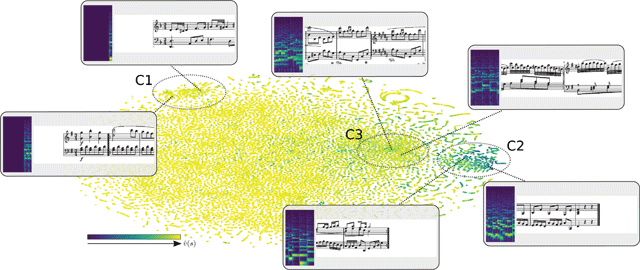
Figure 7
Two-dimensional t-SNE projection of the 512-dimensional embeddings taken from the network’s concatenation layer (see Figure 5). Each point in the scatter plot corresponds to an audio–score input tuple. The color encodes the predicted value ̂v(s;w). (Figure inspired by Mnih et al. (2015).)
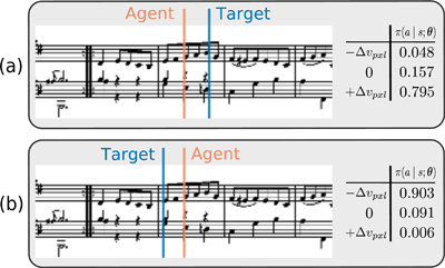
Figure 8
Two examples of policy outputs. (a) Agent is behind the target, resulting in a high probability for increasing the pixel speed (π (+Δνpxl|s;θ) = 0.795). (b) Agent is ahead of the target, suggesting a reduction of pixel speed (π (–Δνpxl|s;θ) = 0.903).
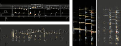
Figure 9
Visualization of the agent’s focus on different parts of the input state for the situation shown in Figure 8b. The salience map was created via integrated gradients (Sundararajan et al., 2017), a technique to identify the most relevant input features for the agent’s decision—in this case, for decreasing its pixel speed.
Table 4
Comparison of score following approaches on real performances. To get a more robust estimate of the performance of the RL agents (REINFORCEbl, A2C and PPO), we report the average over 50 evaluation runs. MM-Loc is the supervised baseline presented by Dorfer et al. (2016). MIDI-ODTW and OMR-ODTW are the ODTW baselines described in Section 4.2. The mean absolute tracking error and its standard deviation are given in centimeters.
| Method | Rtue | Ron | std(|dx|) | |
|---|---|---|---|---|
| Original MIDI Synthesized (Score = Performance) | ||||
| MIDI-ODTW | 1.00 | 1.00 | 0.00 | 0.01 |
| OMR-ODTW | 0.62 | 0.80 | 0.85 | 1.12 |
| MM-Loc | 0.44 | 0.45 | 0.38 | 1.14 |
| REINFORCEbl | 0.56 | 0.59 | 1.15 | 1.14 |
| A2C | 0.70 | 0.63 | 0.65 | 0.82 |
| PPO | 0.74 | 0.68 | 0.7 | 0.87 |
| Performance MIDI Synthesized | ||||
| MIDI-ODTW | 0.81 | 0.94 | 0.50 | 0.76 |
| OMR-ODTW | 0.50 | 0.72 | 0.90 | 1.08 |
| MM-Loc | 0.25 | 0.51 | 0.36 | 0.99 |
| REINFORCEbl | 0.14 | 0.31 | 1.80 | 1.48 |
| A2C | 0.58 | 0.51 | 0.94 | 0.94 |
| PPO | 0.56 | 0.50 | 0.94 | 1.01 |
| Direct Out | ||||
| MIDI-ODTW | 0.88 | 0.92 | 0.59 | 0.79 |
| OMR-ODTW | 0.50 | 0.67 | 0.93 | 1.15 |
| MM-Loc | 0.19 | 0.32 | 0.55 | 1.42 |
| REINFORCEbl | 0.33 | 0.43 | 1.42 | 1.29 |
| A2C | 0.49 | 0.55 | 0.97 | 1.06 |
| PPO | 0.51 | 0.53 | 1.01 | 1.11 |
| Room Recording | ||||
| MIDI-ODTW | 0.81 | 0.93 | 0.64 | 0.84 |
| OMR-ODTW | 0.50 | 0.65 | 0.93 | 1.09 |
| MM-Loc | 0.00 | 0.19 | 0.68 | 1.58 |
| REINFORCEbl | 0.08 | 0.37 | 1.52 | 1.34 |
| A2C | 0.38 | 0.50 | 1.11 | 1.12 |
| PPO | 0.30 | 0.43 | 1.26 | 1.24 |
Table 5
Hyperparameter overview.
| Hyperparameter | Value |
|---|---|
| Adam learning rate | 10–4 |
| Adam decay rates (β1, β2) | (0.9, 0.999) |
| Patience | 50 |
| Learning rate multiplier | 0.1 |
| Refinements | 2 |
| Time horizon tmax | 15 |
| Number of actors | 8 |
| Entropy regularization | 0.05 |
| Discount factor γ | 0.9 |
| GAE parameter λ | 0.95 |
| PPO clipping parameter ɛ | 0.2 |
| PPO epochs | 1 |
| PPO batch size | 120 |
Table 6
Overview of the pieces from the MSMD dataset that were recorded as real performances. The pieces are played without repetitions.
| Composer | Piece name | Dur. (sec.) |
|---|---|---|
| Bach, Johann Sebastian | Polonaise in F major, BWV Anh. 117a | 47.32 |
| Bach, Johann Sebastian | Sinfonia in G minor, BWV 797 | 99.69 |
| Bach, Johann Sebastian | French Suite No. 6 in E major, Menuet, BWV 817 | 37.21 |
| Bach, Johann Sebastian | Partita in E minor, Allemande, BWV 830-2 | 86.73 |
| Bach, Johann Sebastian | Prelude in C major, BWV 924a | 40.43 |
| Bach, Johann Sebastian | Minuet in F major, BWV Anh. 113 | 40.49 |
| Bach, Johann Sebastian | Minuet in G major, BWV Anh. 116 | 51.56 |
| Bach, Johann Sebastian | Minuet in A minor, BWV Anh. 120 | 31.32 |
| Chopin, Frédéric François | Nocturne in B♭ minor, Op. 9, No. 1 | 328.92 |
| Mozart, Wolfgang Amadeus | Piano Sonata No. 11 in A major, 1st Movt, Variation 1, KV331 | 56.33 |
| Mussorgsky, Modest Petrovich | Pictures at an Exhibition, Promenade III | 27.17 |
| Schumann, Robert | Album für die Jugend, Op. 68, 1. Melodie | 45.50 |
| Schumann, Robert | Album für die Jugend, Op. 68, 6. Armes Waisenkind | 73.52 |
| Schumann, Robert | Album für die Jugend, Op. 68, 8. Wilder Reiter | 24.88 |
| Schumann, Robert | Album für die Jugend, Op. 68, 16. Erster Verlust | 55.83 |
| Schumann, Robert | Album für die Jugend, Op. 68, 26. Untitled | 74.40 |