
1 Introduction
Consonance or dissonance, the perceptual effect that is generated by the combination of two or more simultaneous tones, is a fundamental feature of music. More consonant chords are commonly perceived as being more harmonious, smooth or pleasing, whereas dissonant chords are perceived as more unstable, rough or unpleasant. The phenomenon of consonance has been of interest to music theorists since antiquity and has played a prominent role in historical Western theories of harmony (Di Stefano et al., 2022; Hindemith, 1942; Rameau, 1722; Schoenberg, 1948). It is, therefore, unsurprising that a large amount of research has focused on determining the psychological underpinnings for the perception of consonance. Due to its importance in the human listening experience, the ability to accurately characterise perceived consonance or dissonance of chords is crucial for the computational study of music.
Many previous computational approaches for estimating consonance take a perceptual approach in which they aim to simulate possible low‑level psychoacoustic or cognitive processes (Harrison and Pearce, 2020), such as the harmonicity or periodicity of combined sound waves or roughness caused by the interference close overtones. Others (such as Huron, 1994) take something of a hybrid approach by deconstructing a given chord into single intervals, and summing contributions (which may be arrived at through the application of theories of roughness) of consonance or dissonance assigned to each.
The present paper aims to provide computational tools to characterise the simultaneous consonance of symbolic chords, as judged by Western listeners, such as can be represented as collections of notated pitches (or as chord labels, from which pitch classes can be taken). These tools should be flexible, providing computational measures of consonance when there is limited information – such as without knowing chord voicings (the precise placement of pitches within the chord) – and optimised to real‑world behavioural data, rather than testing any particular psychoacoustic theory. Taking a similar approach to Huron (1994), in the present approach, consonance is modelled through the aggregation of contributions of consonance or dissonance for individual pairwise intervals. As well as examining interval values arrived at through theoretical considerations, we compute ideal interval contributions from existing behavioural datasets of chord consonance, as perceived by Western listeners (Bowling et al., 2018; Johnson‑Laird et al., 2012; Popescu et al., 2019). We also investigate the effects on measure performance of the conditional inclusion or exclusion of intervals within chords, thus allowing for more degrees‑of‑freedom in the measures.
1.1 Perceptual models of consonance
Throughout history, many attempts have been made to formally characterise consonance and dissonance. Amongst the earliest numerical approaches, generally attributed to Pythagoras and further formalised by Euler (1739), is the theory that intervals created using simple integer ratios are consonant and those created with more complex ratios are dissonant. Helmholtz (1863/, 1912) took a more explicitly psychoacoustic approach, explaining dissonance as the perceptual roughness created when overtones in complex tones are close but not identical. Stumpf (1890, 1898) suggested that consonance is created through the perceptual merging of overtones within a chord; consonant chords are those that are closer to being perceived as a coherent whole (Schneider, 1997).
Following these early foundations, the majority of current computational attempts to characterise synchronous consonance have taken a perceptual approach. The models produced are formalisations of theories of the perception of consonance through low‑level psychoacoustic features or cognitive processes. Recent comprehensive reviews of consonance research and model comparison are given by Di Stefano et al. (2022) and Harrison and Pearce (2020).1
There are several broad classifications that can be applied to group these models. Theories of chord harmonicity, or periodicity, state that chords are more consonant if their waveform repeats regularly or if their components are more similar to an idealised harmonic series. The concept of consonance for these theories aligns closely with ratio simplicity; chords with simple frequency ratios will have more periodic waveforms. However, formalisations of the harmonicity theory present some difficulties when generalising to chords without just tuning (such as those tuned with equal temperament). Models computing consonance based on the lowest common multiples of ratios can be adapted to give some flexibility in tuning (Stolzenburg, 2015) maximises ratio simplicity with respect to the chord bass notes, allowing intervals to change by about 1% – this step requires that the chord voicing is known). Models computing consonance based on the extent to which a harmonic template fits fundamental pitches and their idealised overtones (and so removing differences in timbre) make use of smoothing to allow for small differences between templates (Harrison and Pearce, 2018; Milne, 2013; Milne et al., 2016).
Following the work of Helmholtz (1863/1912), some models of consonance have sought to characterise the roughness, or interference, experienced when hearing two frequencies in close proximity to each other. If neighbouring overtones of two complex tones are close, without overlapping, roughness may be perceived as dissonance. Of particular relevance to the approach used in this paper are models that formulate a dissonance value for individual pairwise intervals, which are then summed for the chord. This approach applies to several models of roughness, where additive dissonance values are calculated for pairs of frequencies between the overtones (Dillon, 2013; Hutchinson and Knopoff, 1978; Kameoka and Kuriyagawa, 1969; Mashinter, 2006; Plomp and Levelt, 1965; Sethares, 2005). For these models, consonance is purely the absence of any dissonant interactions; adding consonant intervals to a chord will not give a more consonant output.
Rather than using interactions in overtone content, Huron (1994) sums values for intervals in the pitch‑class set of a given chord (Huron initially uses this measure to characterise musical scales; it was then applied to chords by Parncutt et al., 2019). Consonance values for each interval in the octave were created by combining data from three sources (summarised by Krumhansl, 1990, p. 57): the experimental rankings of Malmberg (1918), and the roughness calculation models of Kameoka and Kuriyagawa (1969) and Hutchinson and Knopoff (1978). For each source, interval values were pooled for each interval class and standardised by their means and SDs. Scale directions were adjusted such that consonant intervals were positive. Standardised class scores were then averaged across the three sources. As two of the sources used by Huron (1994) calculate the dissonance of intervals based on the interference between their overtones, the model has been characterised as one of roughness (Harrison and Pearce, 2020; Parncutt et al., 2019). However, it is important to note that the standardisation of values allows for interval contributions to be subtractive, as well as additive. Under this model, the inclusion of more consonant intervals in a chord can mitigate any dissonant intervals.
It has been suggested that the perception of consonance may primarily arise from cultural considerations (Cazden, 1945; McDermott et al., 2016; Omigie et al., 2017; Parncutt and Hair, 2018), counter to theories of consonance as an innate psychoacoustic phenomenon (although these positions are not necessarily irreconcilable, as argued by Di Stefano, 2024). A small number of computational models of consonance have proposed that consonance perception is facilitated through familiarity with musical scales and types of chords. Consonance can be characterised by the extent to which the notes of a chord fit in a diatonic scale (Johnson‑Laird et al., 2012) or the level of exposure a listener has to each chord (Harrison and Pearce, 2020) – the greater familiarity with a chord, the more likely they are to find it consonant.
While these models each aim to provide a measure of consonance according to a specific theory, it is possible that multiple of these theories contribute to the perception of consonance. Harrison and Pearce (2020) present a composite model of consonance. This composite model uses linear contributions from measures of harmonicity (Harrison and Pearce, 2018), roughness (Hutchinson and Knopoff, 1978), cultural familiarity and – optionally – the number of notes in the given chord. The resulting model has been show to more accurately predict behavioural ratings of consonance than models of harmonicity, roughness or cultural familiarity individually (Harrison and Pearce, 2020).
1.2 The present paper
The measures presented in this paper follow the assumption that the consonance of any chord can be characterised by deconstructing it into its constituent intervals – i.e. that the consonance of an interval in isolation does not change when in the presence of other tones. There are compelling arguments against this assumption; Cook (2009, 2017) argues that consonance may also be affected by the location of large and small intervals within chords. However, we believe that the advantage given by the pooling of real‑world data allows this approach to create useful and widely generalisable measures of consonance.
Furthermore, these measures make the assumption that the consonance of chords can be characterised in isolation, in the absence of surrounding musical context. This assumption is also held by the psychoacoustic models discussed above, as well as existing behavioural datasets of consonance. While research suggests that the context of a chord can influence its perceived consonance, we consider this a somewhat separate phenomenon.
As there are multiple viable ways in which such measures may be constructed, we investigate the performance of different methods of aggregation, comparing model fit when summing interval values or averaging them. We hypothesise that the latter will provide a better fit to behavioural data than the former – i.e. that, for larger chord sizes, each individual consonance or dissonance contribution becomes less important.
We compare measures that rely on consonance values for all 12 intervals within an octave and measures that are functions of consonance for interval classes alone. We hypothesise that both methods will provide a close fit to behavioural data but, due to the additional information available, measures using all intervals will perform better.
2 Computational Measures of Consonance
We present a series of computational measures of consonance.2 All measures share the same underlying structure of two parts: First, a value is assigned for each pairwise interval in a given chord that characterises the consonance or dissonance added by the inclusion of that interval; and, second, an aggregation method is applied to combine these values into a single score of consonance. For consistency, we present all measures here as a linear scale between consonance and dissonance, where chords with greater consonance elicit higher positive scores.
The individual consonance values for each interval are taken from a set of weights. In cases in which relative chord voicings are known (e.g. when sufficient inversion information is given), individual weights can be assigned for all 12 pitch intervals in one octave. For a given chord , such that all s are integers (e.g. MIDI pitch values) and , we extract a vector of pairwise intervals (measured in semitones) and denote it by . For each pair of pitches , we assign to a value given by:
To produce measures that are invariant to inversion, we additionally include versions of measures that assign weights for pitch interval classes 0–6. The interval class, in semitones, of the distance between two distinct pitches is defined by:
For example, a measure based on interval classes can be used to characterise the consonance of a chord label. A major chord contains interval classes 3–5, regardless of inversion.
2.1 Measure weights
There are several methods that may be used to obtain weight values. Weights can be assigned based on music‑theoretic principles, such as a simple binary classification with weights of +1 for consonant intervals (or interval classes) and −1 for dissonant intervals.
Distinguishing between the relative consonance and dissonance of intervals, such as by ranking intervals by consonance, allows for more nuanced measures. The work of Malmberg (1918) provides a summary of some of the earliest experimental approaches to the perception of consonance. Seven historical experiments (1897–1918) (Buch, 1900; Faist, 1897; Krueger, 1913; Meinong and Witasek, 1897; Pear, 1911; Stumpf, 1898), with the most thorough conducted by Malmberg (1918), provided ranks for all 12 interval pairs possible within one octave. These ranks are summarised by Schwartz et al. (2003) by taking the median rank across all studies and could function as weights of interval consonance.3 For interval–class weights, the minimum or maximum of the class pair can be considered. Huron (1994) creates a similar set of weights for interval classes through the combination of interval ranks (Malmberg, 1918) and roughness estimates (Hutchinson and Knopoff, 1978; Kameoka and Kuriyagawa, 1969).
Rather than relying on theorised weights, a data‑driven approach may be used to optimise weights from behavioural ratings of chord consonance, providing measures that more closely correspond to real‑world experiences of consonance. We explore and compare measures using both predetermined and optimised weights below.
2.2 Aggregation methods
2.2.1 Sum method
A simple measure of consonance can be produced by summing together weight values for all pairwise intervals in a chord. This method has the property that adding a dissonant interval will produce a linear increase in the absolute dissonance of a chord. Adding one tone to a chord will add multiple pairwise intervals.
We denote by a vector that contains the number of times each interval occurs in . Let denote a vector of weight parameters, with one parameter for each interval. Alternatively, we define the vector of weights as if interval classes are being used.
Using all 12 intervals, we calculate consonance using the sum method as:
It should be noted that this measure is reliant on dissonant chords and weights being negative and on consonant chords and weights positive. This avoids chords becoming characterised as more consonant (or dissonant, were the scale reversed) as chord size increases.
Given average ratings of consonance for distinct chords in a behavioural experiment, weights can be optimised. Let be a vector of centred and scaled perceptual scores between −1 and +1, such that for every ,
where is the most dissonant value of the rating range and the most consonant (i.e. the scale boundaries specified by experimenters, rather than the most extreme values recorded). This implies that a chord at 0 would be perceived as neither consonant nor dissonant.
Weights can be optimised by minimising the sum‑of‑squares objective function:
where is an matrix with rows given by the counts , . The optimisation of over is carried out as follows. First, note that:
Differentiating with respect to yields:
Thus, we conclude that .
It should be noted that this optimisation is equivalent to fitting a multiple linear regression model, in which individual interval counts are each used as features to predict ratings (and without an intercept term). The feature coefficients can be taken as interval weights for the present measures.
2.2.2 Type (weighted mean) method
An alternative approach is to assume that, instead of each interval contributing an absolute value of consonance or dissonance, contributions are relative to the number of intervals in the chord. We produce a measure of consonance by calculating an average of all weights of pairwise intervals in a given chord. More specifically, for a given chord, we calculate the type4 of the vector of intervals, where the type normalises interval counts by the total number of pairwise combinations, such that the type vector sums to 1. Unlike the sum method, this method provides a more conservative measure of consonance for larger chord sizes. The number of interval combinations increases quadratically as a function of the chord size; for type, as chord size increases, the contribution of each interval decreases.
Given a vector of intervals , we denote the type of over the set (or over the set when using interval classes) by . We calculate the type measure of consonance as:
Similarly to the sum method, weights for the type method can be optimised from behavioural data, (this method is invariant to the centring and scaling of data), by minimising the function:
Optimisation of over is given by the closed‑form expression , where is an matrix with rows given by the types , . Alternately, this can be considered a linear regression model using individual interval types as predictors.
2.3 Conditional inclusion of intervals
We may achieve a more flexible measure by splitting the dataset into two complementary parts: chords containing a specific interval , and chords for which is missing. By performing such a split, we are able to assign two sets of weights, one for each subset. Sets of weights can then behave differently based on the inclusion of a particular interval. For example, it is possible that a particular interval allows for distinction between highly consonant and highly dissonant chords, for which interval properties may contribute differently.
We apply this splitting using both the sum and type methods and both interval and interval–class weights. For all possible intervals such that the two subsets are sufficiently large, we fit linear models for individual subsets using the same closed‑form expression as before (i.e. by using interval inclusion as an interaction term).
Further to applying a split based on a single interval, chords can be categorised into four complementary parts: chords containing both intervals , chords containing but not , chords containing but not , and chords for which both and are missing. For both aggregation methods and for each of these four categories, we fit a linear model using the closed‑form expression.
3 Behavioural Datasets
To evaluate the proposed measure, and to optimise weight values, we use data from three existing behavioural studies of consonance perception.5
3.1 Dataset A: Bowling et al. (2018)
In this experiment, 298 distinct chords were each rated by 30 participants, 15 university music students and 15 non‑musicians. During each trial of the experiment, participants heard a single chord, synthesised using a piano sound, and provided a rating of consonance/ dissonance using a four‑point scale (1, ‘quite dissonant’; 2, ‘moderately dissonant’; 3, ‘moderately consonant’; and 4, ‘quite consonant’). Consonance was defined as ‘the musical pleasantness or attractiveness of a sound’. The dataset included all possible two‑, three‑ and four‑note combinations (12 dyads, 66 triads and 220 tetrads) that could be formed using the intervals specified by the chromatic scale over one octave. The register of chords was adjusted such that each chord had a mean F0 of pitches of 263 Hz (C4). For the purposes of the present research, for each chord, we took the mean of participant ratings on the numerical scale above.
It is important to note that, in this experiment, chords were presented using just tuning from the bass note. While the tuning of notes in a chord may affect perceived consonance and is something to which harmonicity models such as Bowling et al. (2018) are sensitive, the measures of the present paper make no distinction between chords using different tuning systems.
Due to its complete coverage of all possible chords of sizes 2–4 within an octave, we use this dataset, centred using Equation 4, to optimise weights for our computational measures of consonance. In total, there is a mean of 127.50 () occurrences for each of the 12 intervals. We use two further datasets to help validate our measures.
3.2 Dataset B: Johnson‑Laird et al. (2012)
In the first of two experiments, consonance ratings were gathered for 55 three‑note chords. These chords contain all 19 different possible pitch‑class set trichords and distinct inversions. Stimuli were synthesised using a piano sound. Each chord was rated by 27 participants (including both musicians and non‑musicians) on a seven‑point scale (1, ‘highly pleasant [consonant]’; 4, ‘neutral’; and 7, ‘highly unpleasant [dissonant]’). In a second experiment, 39 participants rated 43 four‑note chords using the same scale. Chords consisted of either one or two inversions of all 37 possible four‑note pitch class chords, with most chords containing three adjacent semitone intervals excluded. Across both experiments, pitches ranged from G2–G5, with each chord spanning up to two octaves. We took the mean for participant ratings for each chord from both experiments. In this dataset, intervals have a mean count of 41.18 ().
3.3 Dataset C: Popescu et al. (2019)
This study aimed to select chords to function as ‘representative exemplars’ from Classical, Jazz and Avant‑garde musical styles. Twenty chords were selected from real‑world compositions for each style by experts; chords ranged in size from four to eight tones, with a median of five. Across all stimuli, pitches ranged from E1 to C7. An additional 20 five‑note chords randomly generated by sampling uniformly from a chromatic scale spanning four octaves. Each of the 80 chords was presented twice to 30 participants using a piano sound. Participants were not recruited with any requirements of musical background. For each presentation, participants rated chords on two scales: ‘pleasantness’ and ‘roughness’, with the latter explained in terms of compatibility between chord tones (−3, ‘unpleasant’/‘strong roughness’ to +3, ‘pleasant’/‘weak roughness’).
As with the other datasets, we take the mean of participant ratings for each chord. After averaging, ratings for pleasantness and roughness are highly correlated, , . For consistency with definitions of consonance used in the previous datasets, we use the pleasantness scale in our analyses. There are ( occurrences of each interval.
4 Results
We present the results in the following order. First, we present results for measures using weights for all intervals 1–12. This compares the measure output when using both sum and type aggregation methods. Measures are calculated using theoretic binary classification and ranks as weights, then using weights optimised to behavioural data. Second, we present the results for measures using interval classes 0–6, again comparing the output for sum and type variants when using theoretic and optimised weights. Finally, to provide a further point of comparison, we report correlations between several existing computational models of consonance perception and the three datasets. Pearson’s r correlations were calculated for each of the measure variants. This provided a metric of performance that does not depend on the different rating scales used in the behavioural datasets or the output scale of the models.
Dataset A (Bowling et al., 2018) was used to optimise measure‑weights. Due to the possibility of over‑fitting weights to the dataset, particularly for the split measures, with their greater number of optimised parameters, repeated five‑fold cross‑validation was performed. Data were split at random into a training set (80%) and a test set (20%); for each method, we executed 10,000 training–testing rounds, resampling sets each time, and report the means and SDs of r. We also report correlations for the test Datasets B (Johnson‑Laird et al., 2012) and C (Popescu et al., 2019), using weights obtained by optimisation with Dataset A.
Finally, to aid comparison of measures to prior computational models of consonance, we report correlations to test datasets for the best‑performing harmonicity, roughness and cultural‑familiarity models identified by Harrison and Pearce (2020).
4.1 Interval weights
The correlations of full‑interval sum and type measures when using weights of binary classifications and the aggregated historical rankings of Schwartz et al. (2003) are given in Table 1. For the purpose of comparison between variants, this table reports weights and correlations for all measures based on interval data. For consistency between sum and type methods, all weights and behavioural ratings were scaled and centred using Equation 4; −1 indicates the most dissonant value and 1 the most consonant. Both sets of weights produced strong correlations with the behavioural data, with the greater detail afforded by the combined interval ranks of Schwartz et al. (2003) resulting in more accurate models than the binary classifications. Measures using the interval ranks outperformed those using binary classifications for all datasets. For Datasets A and C, the type methods using both sets of weights provided a closer correlation to behavioural ratings than sum; however, the inverse was true for Dataset B.
Table 1
Interval weights and Pearson’s r correlations for cross‑validated (Dataset A, Bowling et al., 2018) and test datasets (B and C, Johnson‑Laird et al., 2012 and Popescu et al., 2019) for sum and type measures.
| Description | Interval | Dataset | ||||||||||||||
|---|---|---|---|---|---|---|---|---|---|---|---|---|---|---|---|---|
| m2 | M2 | m3 | M3 | P4 | TT | P5 | m6 | M6 | m7 | M7 | P8 | A | B | C | ||
| r [SD] | r | r | ||||||||||||||
| Sum method | ||||||||||||||||
| Binary | −1 | −1 | +1 | +1 | +1 | −1 | +1 | +1 | +1 | −1 | −1 | +1 | .592 | .503 | .647 | |
| Schwartz et al. (2003) | −1.0 | −0.4 | 0.0 | +0.4 | +0.6 | −0.2 | +0.8 | +0.2 | +0.4 | −0.4 | −0.8 | +1.0 | .782 | .664 | .745 | |
| Optimised: | ||||||||||||||||
| Simple | −0.39 | −0.04 | −0.01 | +0.05 | +0.14 | −0.12 | +0.15 | −0.08 | −0.03 | −0.14 | −0.20 | +0.24 | .821 [.033] | .703 | .806 | |
| 1‑split | incl. 8 | −0.38 | −0.01 | −0.02 | −0.05 | +0.19 | −0.09 | +0.17 | −0.09 | −0.09 | −0.13 | −0.20 | +0.40 | .824 [.034] | .735 | .787 |
| excl. 8 | −0.39 | −0.08 | −0.01 | +0.13 | +0.13 | −0.15 | +0.14 | – | +0.01 | −0.18 | −0.19 | +0.23 | ||||
| 2‑split | in. 4, in. 8 | −0.53 | −0.05 | −0.12 | −0.16 | +0.40 | −0.02 | +0.23 | +0.11 | −0.18 | −0.22 | −0.07 | +0.35 | .810 [.038] | .734 | .732 |
| in. 4, ex. 8 | −0.44 | −0.05 | −0.01 | +0.10 | +0.18 | −0.15 | +0.20 | – | −0.01 | −0.15 | −0.24 | +0.22 | ||||
| ex. 4, in. 8 | −0.31 | +0.03 | +0.09 | – | +0.08 | −0.14 | +0.06 | −0.12 | −0.09 | −0.11 | −0.28 | +0.13 | ||||
| ex. 4, ex. 8 | −0.32 | −0.15 | +0.02 | – | +0.15 | −0.19 | +0.13 | – | +0.02 | −0.20 | −0.20 | +0.24 | ||||
| Type method | ||||||||||||||||
| Binary | −1 | −1 | +1 | +1 | +1 | −1 | +1 | +1 | +1 | −1 | −1 | +1 | .645 | .494 | .725 | |
| Schwartz et al. (2003) | −1.0 | −0.4 | 0.0 | +0.4 | +0.6 | −0.2 | +0.8 | +0.2 | +0.4 | −0.4 | −0.8 | +1.0 | .804 | .640 | .740 | |
| Optimised: | ||||||||||||||||
| Simple | −1.90 | −0.30 | −0.03 | +0.26 | +0.62 | −0.58 | +0.68 | −0.34 | −0.14 | −0.71 | −0.90 | +1.01 | .835 [.039] | .676 | .837 | |
| 1‑split | incl. 8 | −2.35 | −0.17 | −0.28 | −0.48 | +1.03 | −0.61 | +0.91 | +0.01 | −0.47 | −0.90 | −1.27 | +2.08 | .851 [.036] | .732 | .829 |
| excl. 8 | −1.76 | −0.41 | −0.03 | +0.47 | +0.50 | −0.67 | +0.69 | – | +0.03 | −0.78 | −0.80 | +0.85 | ||||
| 2‑split | in. 4, in. 8 | −3.18 | −0.26 | −0.67 | −0.74 | +2.44 | −0.06 | +1.43 | +0.26 | −0.97 | −1.25 | −0.31 | +2.05 | .856 [.034] | .739 | .780 |
| in. 4, ex. 8 | −2.55 | −0.22 | −0.02 | +0.51 | +1.08 | −0.84 | +1.15 | – | −0.14 | −0.70 | −1.51 | +1.34 | ||||
| ex. 4, in. 8 | −1.95 | −0.00 | +0.35 | – | +0.38 | −0.96 | +0.23 | +0.03 | −0.58 | −0.88 | −1.86 | +0.67 | ||||
| ex. 4, ex. 8 | −1.49 | −0.54 | +0.06 | – | +0.44 | −0.65 | +0.59 | – | −0.10 | −0.75 | −0.77 | +0.81 | ||||
4.1.1 Optimised interval weights
For both the sum (Equation 3) and type (Equation 11) methods, interval weights were optimised by minimising the sum‑of‑squares functions (Equations 5 and 12, respectively), using Dataset A and five‑fold cross‑validation. The optimised weight values and mean correlations with behavioural data are given in Table 1 (‘simple’). For both methods, optimised weights performed better than the binary and ranked values, across all datasets. The type method was the better‑performing one for Datasets A and C; sum more closely matched the participant ratings of Dataset B.
4.1.2 Conditional inclusion of a specific interval
The conditional inclusion of a specific interval assigned chords to two categories: chords that contained the interval and chords from which it was absent. Sets of weights were optimised for both categories. Correlations were calculated between measure values for each given chord (using the relevant weights) and behavioural ratings. While the conditional inclusion of several intervals provided higher correlations to behavioural datasets than the single set of optimised weights, no one interval consistently provided an improvement across all datasets and aggregation methods. For completeness, Table 2 shows the mean cross‑validated training correlations and test dataset correlations for this measure when including/excluding all intervals . Splitting data based on interval 8 (m6) provided the best correlations with Dataset B. Table 1 reports the weights and correlations for this variant (these weights, and those of the ‘simple’ optimisation are shown in Figure 1); however, there are other viable options which may be selected based on other criteria. This measure improved on the performance of the ‘simple’ optimised weights for both sum and type for Datasets A and B. The type method provided a closer fit to Datasets A and C than the sum method.
Table 2
Pearson’s r correlations between behavioural datasets and sum and type measures based on the conditional inclusion of a specific interval. Column n–✓ gives the number of chords in Dataset A (Bowling et al., 2018) that contain interval i. Correlations that are higher than the previous ‘simple’ optimised weights, for each method and dataset, are shown in bold.
| Dataset A | B | C | ||||||||
|---|---|---|---|---|---|---|---|---|---|---|
| n | Sum | Type | Sum | Type | Sum | Type | ||||
| i: | ✓ | x | r | SD | r | SD | r | r | r | r |
| 1 | 158 | 140 | .835 | .035 | .857 | .036 | .665 | .662 | .754 | .816 |
| 2 | 150 | 148 | .835 | .034 | .819 | .045 | .722 | .683 | .745 | .822 |
| 3 | 142 | 156 | .811 | .034 | .841 | .036 | .698 | .666 | .797 | .821 |
| 4 | 134 | 164 | .826 | .033 | .856 | .036 | .721 | .707 | .773 | .822 |
| 5 | 125 | 173 | .820 | .033 | .835 | .038 | .685 | .666 | .808 | .854 |
| 6 | 117 | 181 | .814 | .034 | .829 | .039 | .700 | .684 | .795 | .842 |
| 7 | 117 | 181 | .812 | .035 | .830 | .040 | .685 | .668 | .800 | .826 |
| 8 | 107 | 191 | .824 | .034 | .851 | .036 | .735 | .732 | .787 | .829 |
| 9 | 97 | 201 | .818 | .032 | .834 | .037 | .711 | .670 | .777 | .820 |
| 10 | 87 | 211 | .825 | .036 | .825 | .042 | .684 | .647 | .755 | .825 |
| 11 | 77 | 221 | .820 | .036 | .829 | .042 | .710 | .665 | .746 | .832 |
| 12 | 67 | 231 | .809 | .036 | .827 | .039 | .718 | .681 | .761 | .818 |
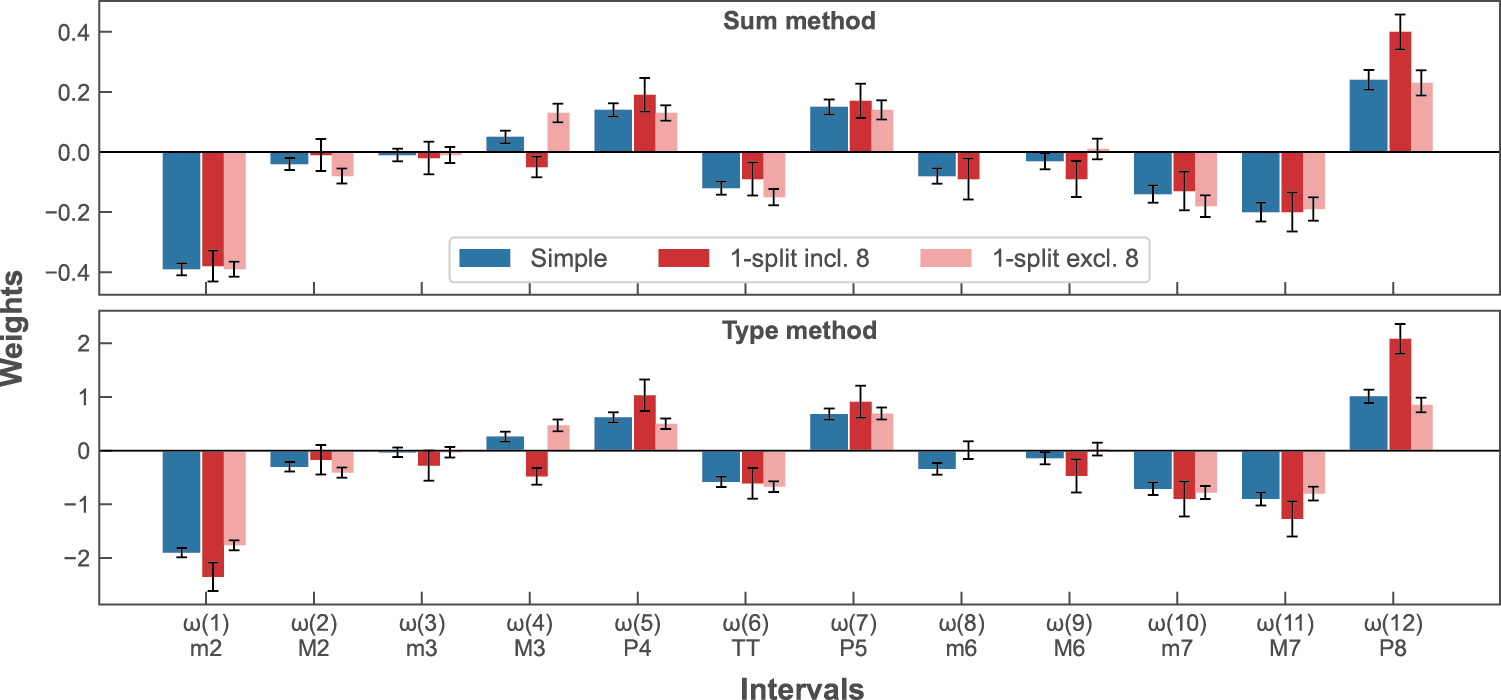
Figure 1
‘Simple’ and 1‑split (including/excluding m6) optimised interval weights for sum and type measures. Error bars display the standard errors of optimised weights.
4.1.3 Conditional inclusion of interval pairs
Further measures conditionally assigned chords to four complementary categories based on pairs of intervals (i and j): chords that included i and j, chords that included i but not j, chords that included j but not i and chords that included neither. As with the previous optimisations, we performed five‑fold cross‑validation. For each pair, the linear models of Equations 5 and 12 were fitted using the closed‑form expression . Since at least one of the four training subsets could contain relatively few samples, we encountered ill‑posed problems – i.e. the determinant of the matrix was zero or extremely small. To overcome this obstacle, 10,000 training–testing rounds were executed; only interval pairs for which at least 5,000 rounds were completed successfully for both the sum and type methods were considered (57 out of 66 pairs). We report the averages of correlation coefficients from all successful rounds (5,000–10,000 for each interval pair).
Details of the two best‑performing interval pairs for each dataset are reported in Table 3 (for results of all possible pairs, see Supplementary Materials, Table A1). The conditional inclusion/exclusion of some interval pairs produced closer fits to behavioural data than those of Table 2; however, many of these improvements are for the training Dataset A and so should be considered with caution. Categorising data based on intervals 4 (M3) and 8 (m6) provided the best correlations with Dataset B and is shown in Table 1. Figure 2 illustrates (on the left) the relationship between the behavioural datasets and sum and type measures using these weights and (on the right) the relationship between individual categories and Dataset A. As with the previous optimised results, the type method largely provided a closer fit to Datasets A and C than the sum method; however, this is not the case for Dataset B.
Table 3
Pearson’s r correlations between behavioural datasets and best‑performing sum and type measures based on the conditional inclusion of pairs of intervals. Column n–✓–✓ gives the number of chords in Dataset A that contain both intervals i and j. Correlations that are higher than the best‑performing measure of Table 2, for each method and dataset, are shown in bold.
| Dataset A | B | C | |||||||||||
|---|---|---|---|---|---|---|---|---|---|---|---|---|---|
| n | Sum | Type | Sum | Type | Sum | Type | |||||||
| i: | ✓ | ✓ | × | × | r | SD | r | SD | r | r | r | r | |
| j: | ✓ | × | ✓ | × | |||||||||
| 1 | 3 | 77 | 81 | 65 | 75 | .818 | .040 | .858 | .035 | .660 | .660 | .712 | .774 |
| 1 | 4 | 71 | 87 | 63 | 77 | .833 | .034 | .871 | .032 | .674 | .690 | .745 | .817 |
| 1 | 8 | 59 | 99 | 48 | 92 | .854 | .031 | .873 | .030 | .639 | .701 | .686 | .797 |
| 1 | 9 | 54 | 104 | 43 | 97 | .842 | .033 | .848 | .038 | .652 | .639 | .721 | .789 |
| 2 | 4 | 57 | 93 | 77 | 71 | .821 | .036 | .831 | .043 | .746 | .696 | .737 | .813 |
| 2 | 6 | 62 | 88 | 55 | 93 | .823 | .036 | .812 | .043 | .736 | .706 | .741 | .808 |
| 2 | 10 | 49 | 101 | 38 | 110 | .838 | .037 | .807 | .049 | .699 | .648 | .688 | .788 |
| 3 | 5 | 63 | 79 | 62 | 94 | .808 | .035 | .840 | .036 | .659 | .646 | .806 | .852 |
| 4 | 8 | 43 | 91 | 64 | 100 | .810 | .038 | .856 | .034 | .734 | .739 | .732 | .780 |
| 5 | 8 | 36 | 89 | 71 | 102 | .819 | .035 | .856 | .032 | .705 | .699 | .786 | .851 |
| 6 | 8 | 35 | 82 | 72 | 109 | .810 | .037 | .845 | .034 | .717 | .727 | .769 | .795 |
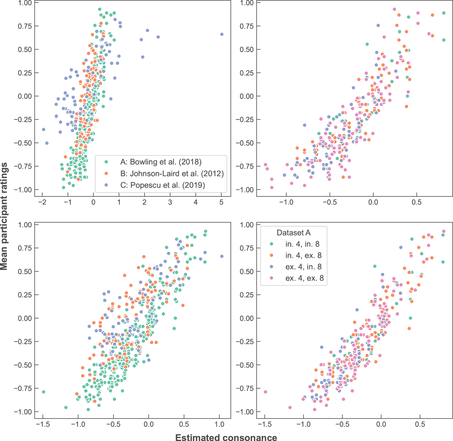
Figure 2
Perceptual vs. estimated scores for interval measures based on the inclusion/exclusion of intervals 4 and 8. Left: comparison between Datasets A, B and C (Bowling et al., 2018; Johnson‑Laird et al., 2012; Popescu et al., 2019) for the sum (top) and type methods (bottom). Right: the four clusters of Dataset A, based on the inclusion/exclusion of intervals 4 and 8, for the sum (top) and type methods (bottom).
4.2 interval–class weights
Correlations between behavioural datasets and sum and type measures using interval–class weights are given in Table 4.6 As with interval results, this table allows for comparison between all measure variants using interval–classes. As Schwartz et al. (2003) provides rankings for all intervals, the minima and maxima of interval–class pairs were both tested. For both aggregation methods, choosing the lower – more dissonant – weight of interval–class pairs provided a better fit with behavioural data (with the exception of sum and Dataset C). Even though the interval–class measures are more limited in information than those using weights for all intervals, the type method using the lower class weights of Schwartz et al. (2003) matched or improved on the fit of the interval measures for all datasets.
Table 4
Interval–class weights and Pearson’s r correlations for cross‑validated (Dataset A, Bowling et al., 2018) and test datasets (B and C, Johnson‑Laird et al., 2012; Popescu et al., 2019) for sum and type measures.
| Description | Interval class | Dataset | |||||||||
|---|---|---|---|---|---|---|---|---|---|---|---|
| P1/P8 | m2/M7 | M2/m7 | m3/M6 | M3/m6 | P4/P5 | TT | A | B | C | ||
| r [SD] | r | r | |||||||||
| Sum method | |||||||||||
| Binary | +1 | −1 | −1 | +1 | +1 | +1 | −1 | .587 | .503 | .647 | |
| Schwartz et al. (2003): | |||||||||||
| Class max. | +1.0 | −0.8 | −0.4 | +0.4 | +0.4 | +0.8 | −0.2 | .733 | .623 | .782 | |
| Class min. | +1.0 | −1.0 | −0.4 | 0.0 | +0.2 | +0.6 | −0.2 | .791 | .661 | .761 | |
| Huron (1994) | – | −1.43 | −0.58 | +0.59 | +0.39 | +1.24 | −0.45 | .703 | .680 | .739 | |
| Optimised: | |||||||||||
| Simple | +0.25 | −0.34 | −0.08 | −0.02 | −0.00 | +0.15 | −0.11 | .796 [.038] | .704 | .788 | |
| 1‑split | incl. 4 | +0.34 | −0.37 | −0.05 | −0.01 | −0.05 | +0.22 | −0.09 | .808 [.037] | .751 | .765 |
| excl. 4 | +0.25 | −0.27 | −0.18 | +0.02 | – | +0.14 | −0.20 | ||||
| 2‑split | in. 4, in. 6 | +0.36 | −0.32 | −0.02 | −0.01 | −0.06 | +0.15 | −0.10 | .801 [.039] | .757 | .760 |
| in. 4, ex. 6 | +0.33 | −0.35 | −0.07 | −0.01 | −0.07 | +0.25 | – | ||||
| ex. 4, in. 6 | +0.33 | −0.36 | +0.02 | −0.01 | – | +0.11 | −0.16 | ||||
| ex. 4, ex. 6 | +0.25 | −0.24 | −0.21 | −0.01 | – | +0.18 | – | ||||
| Type method | |||||||||||
| Binary | +1 | −1 | −1 | +1 | +1 | +1 | −1 | .645 | .494 | .725 | |
| Schwartz et al. (2003): | |||||||||||
| Class max. | +1.0 | −0.8 | −0.4 | +0.4 | +0.4 | +0.8 | −0.2 | .779 | .623 | .711 | |
| Class min. | +1.0 | −1.0 | −0.4 | 0.0 | +0.2 | +0.6 | −0.2 | .802 | .643 | .802 | |
| Huron (1994) | – | −1.43 | −0.58 | +0.59 | +0.39 | +1.24 | −0.45 | .722 | .656 | .771 | |
| Optimised: | |||||||||||
| Simple | +1.03 | −1.57 | −0.49 | −0.09 | +0.00 | +0.67 | −0.56 | .804 [.046] | .683 | .818 | |
| 1‑split | incl. 4 | +1.64 | −2.17 | −0.37 | −0.10 | −0.08 | +1.21 | −0.56 | .835 [.037] | .731 | .807 |
| excl. 4 | +0.83 | −1.21 | −0.67 | +0.00 | – | +0.52 | −0.68 | ||||
| 2‑split | in. 4, in. 6 | +1.61 | −2.01 | −0.20 | −0.17 | −0.44 | +0.77 | −0.13 | .833 [.038] | .747 | .812 |
| in. 4, ex. 6 | +1.54 | −2.12 | −0.44 | −0.10 | −0.12 | +1.34 | – | ||||
| ex. 4, in. 6 | +0.80 | −2.04 | −0.70 | −0.03 | – | +0.76 | −0.39 | ||||
| ex. 4, ex. 6 | +0.77 | −1.08 | −0.72 | −0.05 | – | +0.65 | – | ||||
Here, we also include the interval–class values of Huron (1994) as weights for sum and type methods. Although similar to the sum method, the original model summed values for pairwise intervals of a chord’s pitch class set, rather than for all interval classes that actually occur. It should also be noted that Huron (1994) ignores unison and octave intervals. The sum method provided an identical or better fit to behavioural data than the original model (see Table 7 for correlations of previous perceptual models to behavioural datasets).
4.2.1 Optimised interval–class weights
As with measures using interval weights, interval–class weights were optimised for sum and type methods by minimising Equations 5 and 12 using behavioural Dataset A and five‑fold cross‑validation. The weights and correlations obtained for this ‘simple’ optimisation are reported in Table 4. Measures using optimised weights provided a better fit to behavioural data than the weights obtained from Schwartz et al. (2003) and Huron (1994). The type method provided a better fit than the sum method for Datasets A and C. As would be expected, the reduced number of parameters being optimised resulted in lower correlations to behavioural data than the equivalent measures using all 12 intervals.
4.2.2 Conditional inclusion of a specific interval class
Weights were optimised using the conditional inclusion or exclusion of each of the interval classes 0–6. Correlations to behavioural datasets are shown in Table 5. The conditional inclusion of many interval classes increased measure performance over the ‘simple’ version, particularly for Dataset B (all variants provided a better fit except the type method when including/excluding class 5, P4/P5); however, there was little improvement for Dataset C. As with the interval measures, we report in Table 4 and Figure 3 the weights for the sum and type when including/excluding class 4 (M4/m6) – the class that provided the best fit to Dataset B. There was some consistency between interval and interval–class measures, with interval 8 (see in Table 1) belonging to interval class 4. In general, type provided closer correlations to Datasets A and C, whereas sum provided closer correlations to Dataset B.
Table 5
Pearson’s r correlations between behavioural datasets and sum and type measures based on the conditional inclusion of a specific interval class. Correlations that are higher than the previous ‘simple’ optimised weights, for each method and dataset, are shown in bold.
| Dataset A | B | C | ||||||||
|---|---|---|---|---|---|---|---|---|---|---|
| n | Sum | Type | Sum | Type | Sum | Type | ||||
| i: | ✓ | × | r | SD | r | SD | r | r | r | r |
| 0 | 67 | 231 | .787 | .041 | .800 | .046 | .721 | .694 | .744 | .817 |
| 1 | 188 | 110 | .813 | .041 | .843 | .038 | .715 | .693 | .736 | .782 |
| 2 | 188 | 110 | .828 | .037 | .794 | .048 | .738 | .687 | .723 | .816 |
| 3 | 187 | 111 | .787 | .039 | .816 | .039 | .711 | .692 | .781 | .822 |
| 4 | 198 | 100 | .808 | .037 | .835 | .037 | .751 | .731 | .765 | .807 |
| 5 | 188 | 110 | .796 | .038 | .816 | .041 | .713 | .679 | .785 | .811 |
| 6 | 117 | 181 | .795 | .037 | .807 | .042 | .712 | .706 | .782 | .829 |
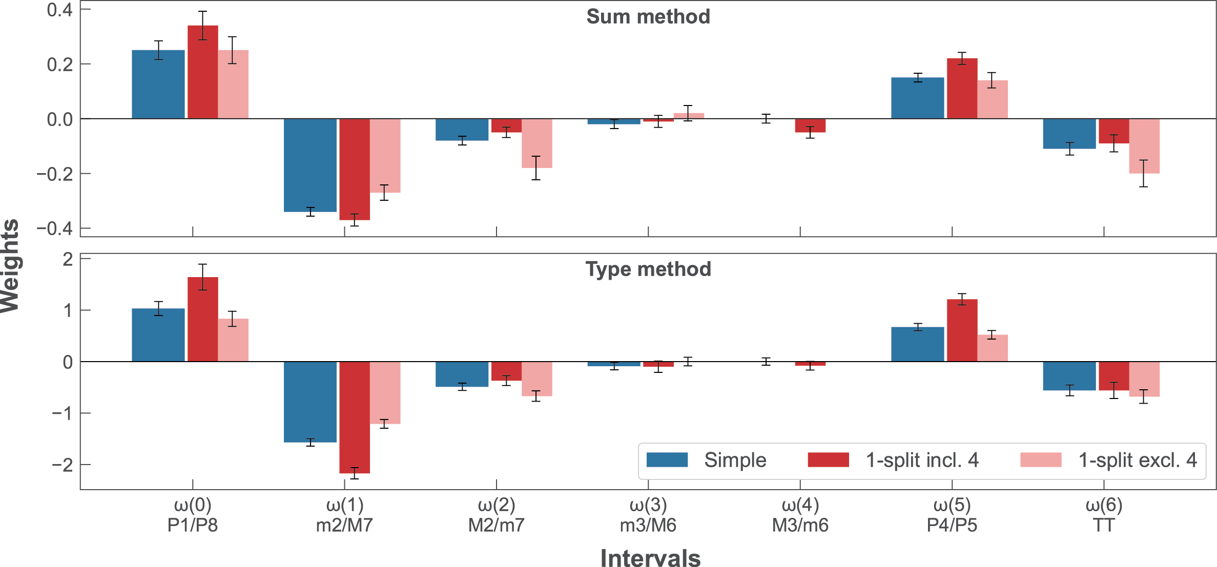
Figure 3
‘Simple’ and 1‑split (including and excluding M3/m6) optimised interval–class weights for sum and type measures. Error bars display the standard errors of optimised weights.
4.2.3 Conditional inclusion of interval–class pairs
Weights sets were optimised based on the conditional inclusion of two interval classes. As with the previous optimisation of weights based on the conditional inclusion of two intervals, repeated five‑fold cross‑validation was used. interval–class pairs were only considered if at least 5,000 of the 10,000 repetitions were completed successfully for both sum and type methods (nine pairs failed this test). Table 6 shows the correlations between behavioural datasets and the best two performing interval–class combinations for each dataset (see Supplementary Materials, Table A2, for all possible pairs). Measures based on the inclusion/exclusion of pairs of classes produced only limited improvements over single‑class and simple versions. Categorising chords based on classes 4 (M3/m6) and 6 (TT) was the variant with the best fit to Dataset B (and was the only one to improve for both sum and type). The weights for this measure are given in Table 4. The relationships between the behavioural datasets and measures using these weights are displayed in Figure 4 (left) and between chord categories and Dataset A (right).
Table 6
Pearson’s r correlations between behavioural datasets and best‑performing sum and type measures based on the conditional inclusion of pairs of interval classes. Correlations that are higher than the best‑performing measure of Table 5, for each method and dataset, are shown in bold.
| Dataset A | B | C | |||||||||||
|---|---|---|---|---|---|---|---|---|---|---|---|---|---|
| n | Sum | Type | Sum | Type | Sum | Type | |||||||
| ✓ | ✓ | × | × | r | SD | r | SD | r | r | r | r | ||
| i: | j: | ✓ | × | ✓ | × | ||||||||
| 0 | 2 | 29 | 38 | 159 | 72 | .830 | .041 | .790 | .049 | .750 | .693 | .610 | .774 |
| 0 | 4 | 30 | 37 | 168 | 63 | .794 | .045 | .826 | .041 | .760 | .730 | .628 | .794 |
| 1 | 3 | 128 | 60 | 59 | 51 | .824 | .036 | .857 | .033 | .740 | .712 | .699 | .762 |
| 1 | 4 | 132 | 56 | 66 | 44 | .822 | .038 | .857 | .035 | .737 | .726 | .729 | .800 |
| 1 | 5 | 130 | 58 | 58 | 52 | .818 | .036 | .865 | .030 | .731 | .705 | .737 | .800 |
| 2 | 4 | 124 | 64 | 74 | 36 | .825 | .036 | .830 | .040 | .765 | .730 | .740 | .820 |
| 2 | 5 | 114 | 74 | 74 | 36 | .827 | .039 | .805 | .045 | .739 | .686 | .728 | .798 |
| 3 | 4 | 132 | 55 | 66 | 45 | .816 | .036 | .833 | .038 | .755 | .733 | .771 | .815 |
| 3 | 5 | 128 | 59 | 60 | 51 | .797 | .037 | .833 | .035 | .717 | .691 | .786 | .819 |
| 3 | 6 | 55 | 132 | 62 | 49 | .783 | .042 | .818 | .036 | .735 | .711 | .773 | .823 |
| 4 | 6 | 82 | 116 | 35 | 65 | .801 | .039 | .833 | .038 | .757 | .747 | .760 | .812 |
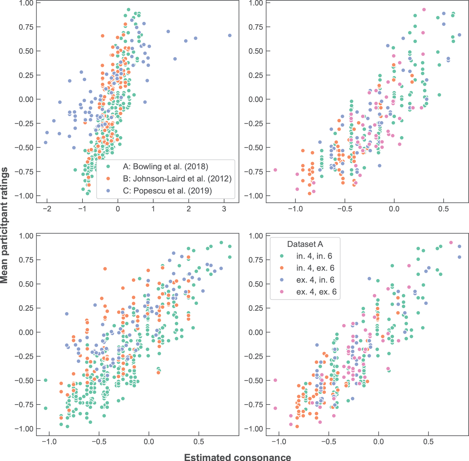
Figure 4
Perceptual vs. estimated scores for interval–class measures based on the inclusion/exclusion of classes 4 and 6. Left: comparison between the three datasets (Bowling et al., 2018; Johnson‑Laird et al., 2012; Popescu et al., 2019) for the sum (top) and type methods (bottom). Right: the four clusters of dataset Bowling et al. (2018), based on the inclusion/exclusion of intervals 4 and 8, for the sum (top) and type methods (bottom).
4.3 Performance of perceptual models
To aid the comparison of measures to previous computational models of consonance, we include Table 7. Correlations were computed between datasets and the two best‑performing harmonicity (Harrison and Pearce, 2018; Stolzenburg, 2015), roughness (Huron, 1994; Hutchinson and Knopoff, 1978) and cultural‑familiarity models (Harrison and Pearce, 2020; Johnson‑Laird et al., 2012), as evaluated by Harrison and Pearce (2020), as well as their composite model.7 In comparing models, it is worth noting that the different models use different levels of chord information as their input. The models Harrison and Pearce (2018) and Huron (1994) use only pitch classes of given chords, whereas Stolzenburg (2015), Hutchinson and Knopoff (1978), Johnson‑Laird et al. (2012) and Harrison and Pearce (2020) require information on chord voicings. The former models are, therefore, best compared to sum and type measures using interval classes, and the latter to measures using all intervals.
Table 7
Pearson r correlations of perceptual models of consonance to behavioural datasets. Highest correlations for each dataset are shown in bold for perceptual models and for the measures of the present paper displayed.
| Model | Description | Dataset r | ||
|---|---|---|---|---|
| A | B | C | ||
| Perceptual models | ||||
| Harrison and Pearce (2018) | harmonicity | .620 | .496 | .706 |
| Stolzenburg (2015) | harmonicity | .740 | .723 | .785 |
| Huron (1994) | roughness | .685 | .680 | .650 |
| Hutchinson and Knopoff (1978) | roughness | .713 | .440 | .550 |
| Johnson‑Laird et al. (2012) | cultural | .634 | .719 | .725 |
| Harrison and Pearce (2020) | cultural | .722 | .568 | .850 |
| Harrison and Pearce (2020) | composite | .801 | .628 | .830 |
| Optimised models | ||||
| Simple: | ||||
| Interval | sum | .821 | .703 | .806 |
| type | .835 | .676 | .837 | |
| Interval class | sum | .796 | .704 | .788 |
| type | .804 | .683 | .818 | |
| 1‑split: | ||||
| Interval (incl./excl. 8) | sum | .824 | .735 | .787 |
| type | .851 | .732 | .829 | |
| Interval class (incl./excl. 4) | sum | .808 | .751 | .765 |
| type | .835 | .731 | .807 | |
5 Discussion
The research presented in this paper aimed to construct and compare measures of simultaneous chord consonance and dissonance. In particular, these measures aimed to model consonance in cases where only limited information is available, such as given by chord labels where voicings are unknown. Measures sought to assign a value for each pairwise interval in a chord that characterised the consonance or dissonance created by its inclusion. Pairwise consonance weights were then aggregated, with sum and type methods compared.
5.1 Sum and type aggregation methods
The two approaches of combining interval weights imply subtle differences as to how individual pairwise intervals contribute to the perceived consonance and dissonance of chords. For the sum method, individual intervals contribute an absolute value of consonance or dissonance; consonant intervals are additive to the output and dissonant ones subtractive. Weights are not scaled by chord size – measure values are comparable for different chord sizes due to the balance between consonant and dissonant weights. This measure follows the hypothesis that inclusion of intervals contributes linearly to consonance or dissonance. In contrast, summing the type, or empirical distribution, for each interval category over all pairwise combinations in the chord provides weights that are relative to the mean for that chord. Adding intervals with weights equal to the mean will not change a chord’s consonance; a weight of zero will change the overall chord consonance unless it is also the mean (unlike for sum). As chord size increases, the contribution of each interval diminishes.
For both interval and interval–class measures, the type method provided a closer fit to behavioural Datasets A (Bowling et al., 2018) and C (Popescu et al., 2019) than those using sum. These modest improvements were produced both when using weights optimised from data and when using weights formed from ranking intervals. Dataset B (Johnson‑Laird et al., 2012), however, produced an opposite effect, with the sum method providing the better performance.
5.2 Interval and interval–class weights
We presented computational measures using two types of weights: first, using the 12 chromatic intervals within an octave; second, using seven interval classes. The aim of the latter was to allow for measures of consonance that did not use any information about chord voicing. One substantial difference between these versions, therefore, is that those using interval can account for different inversions of the same chord, while those using interval class cannot. Previous empirical evidence suggests there are significant differences in the perception of consonance for chords in different inversions; root position chords are perceived as more consonant (Johnson‑Laird et al., 2012; Roberts, 1986).
The reduction of the full 12 interval weights to seven interval classes generally resulted in weaker correlations between measures and behavioural data. This is not surprising given the extra information available when using interval weights, particularly for optimised variants, and the previous empirical findings; however, the performance gap between interval and interval–class weights is small. There were several cases where interval–class measures performed comparably with those of interval. When using the rankings of Schwartz et al. (2003) – taking the most dissonant ranking for each interval–class pair – to predict ratings for the three test datasets, both sum and type (with the exception of Dataset C) gave a closer fit than those using the full 12 rankings.
The results reveal some interesting differences in the perception of consonance between intervals in isolation and intervals within chords. The interval rankings of Schwartz et al. (2003) show differences in consonance between intervals and their inverted counterparts; with the exception of the M3, larger intervals have more consonant ranks (M2 and m7 are equal). When combined across pairwise intervals, these rankings would imply that second‑inversion major triads and first‑inversion minor triads are perceived as more consonant than in their root positions. However, the optimised weights for both sum and type methods differ from the ranks of Schwartz et al. While M7 is substantially less dissonant than m2, and P5 more consonant than P4, the intervals of M2, m3 and M3 are all the more consonant of their respective classes. For these weights, root position triads gain a more consonant score than their inversions.
5.3 Conditional inclusion of intervals and interval classes
We hypothesised that conditionally categorising chords based on the inclusion or exclusion of a given interval, giving one set of weights for chords that contain the interval and another set for chords that do not, would improve the fit of the measures to behavioural data. This approach allows us to determine whether certain intervals change how consonance is perceived – or rather, whether certain intervals indicate particular types of chords, for which consonance and dissonance are perceived differently. For example, it is possible that a distinction is made between highly consonant and highly dissonant chords, for which interval properties contribute differently. A particularly interesting extension of this distinction would be between cluster chords and dissonant chords created through the extension of triads.
There is some evidence for this behaviour in the single‑interval results for both interval and interval–class (Tables 2 and 5, respectively). Categorising chords based on the inclusion/exclusion of m2 substantially improved on the fit of the ‘simple’ optimised weights for Dataset A, indicating some advantage to clustering chords based on dissonance. Categorisations based on M3 and m6 (both interval class 4) provide a better fit than the simple optimised weights for both Datasets A and B. The presence of a, M3 in a chord may provide enough of an indication that the chord has a triadic base for a distinction of chord type to take place. A further distinction of chord inversion may also be influencing the model output, leading to the conditional inclusion of m6, producing high correlations with behavioural data.
We reported the results when including or excluding interval 8 (m6) and interval class 4 in Tables 1 and 4. These measures had the best performance in predicting Dataset B; however, several other intervals present plausible options.
We also reported findings for measures based on the conditional inclusion of two intervals or classes. This allowed us to investigate the extent to which the more nuanced classifications aided the modelling of consonance. As shown in Tables 3 and 6, while these models produce some performance gains for individual intervals, methods and datasets, they do not convincingly offer any general improvement, and a single optimal solution is difficult to identify. It is possible that this lack of consistency between results is due to the reduced data available for training weights when splitting the dataset into four categories.
The combination of intervals 4 and 8 (M3 and m6), most closely fitting Dataset B, provides further evidence that the most effective interval categorisations help to characterise triadic and non‑triadic chords. Interval classes of 4 and 6 likewise could be produced by the classification of triadic and highly‑dissonant chords.
5.4 Measure selection
Out of the variants compared in this paper, several are viable candidates for the best measure of consonance. In many cases, the optimal choice will be dependant on the particular application; while interval–class measures performed well, using 12 interval weights offers a more nuanced measure of consonance, if the information is available. In general, measures based on the conditional inclusion of a single interval/class (interval m6 or interval class M3/m6), using the type method (particularly when modelling larger chords), seem to offer the best balance between performance and complexity. However, the ‘simple’ set of optimised weights may provide a more robust measure in some cases.
5.5 Perceptual models of consonance
It is not intended that the measures presented in this paper should perform as indicators of cognitive or psychoacoustic processes, such as models based on theories of harmonicity (Harrison and Pearce, 2018; Stolzenburg, 2015), roughness (Huron, 1994; Hutchinson and Knopoff, 1978) and cultural familiarity (Harrison and Pearce, 2020; Johnson‑Laird et al., 2012). However, as computational tools of consonance characterisation, perceptual models of cognition provide a useful point of comparison.
As shown by Table 7, models based on perceptual theories of consonance generally fit the behavioural datasets well, particularly the periodicity model of Stolzenburg (2015), and the cultural (excluding Dataset B) and composite models of Harrison and Pearce (2020). These three models all make use of some voicing information – Stolzenburg (2015) adjusts chord tuning to bass pitches, while Harrison and Pearce (2018) count occurrences of chords represented as pitch‑class sets relative to the bass which, along with the roughness model of Hutchinson and Knopoff (1978), is inherited by the composite model – and so provide the most direct comparisons to sum and type measures using interval weights. Interval measures, particularly when optimised based on the conditional inclusion of m6 using type, provide a better fit to Datasets A and B. The high correlation between the cultural‑familiarity model of Harrison and Pearce (2020) and Dataset C, which both used chords that are more representative of those present in real‑world corpora, suggests that better measure performance could be achieved if weights were optimised from a large dataset of real‑world chords and behavioural ratings.
For these datasets, models that discard voicing information by using pitch‑class sets (Huron, 1994; Harrison and Pearce, 2018) produced lower correlations. In comparison, measures using interval–class weights produced only marginally lower correlations than those using all 12 intervals. Of particular interest is the comparison between the model of Huron (1994) as originally formulated using pitch‑class sets (used in Table 7), the sum and type aggregations using Huron’s weights over all interval classes and measures using optimised data. Table 4 shows that summing weights for all pairwise interval classes, rather than pitch‑class sets, improves model performance. As previously discussed, the type method fits more closely Datasets A and C than summing weights, as used in Huron (1994). The measures using optimised weights out‑perform those using the Huron’s weights for all test datasets. However, it is possible that some of this difference is due to Huron (1994) omitting any consonance contributions of octaves (the model was originally formulated to characterise consonance of scales, rather than chords).
Although the sum and type measures are not strictly measures of a specific theory of perception, they can still provide some useful insights as to how consonance is perceived. Under the assumption that consonance perception (or, at least a substantial factor of consonance perception) can be attributed to the relationships between individual pairwise intervals in chord (see Cook, 2009, Cook, 2017 for counter‑arguments), the interval weights obtained from optimisation to behavioural data give information about their relative differences in consonance.
For the sum method weights, negative weights are those that increase the dissonance of a chord, whereas positive weights increase its consonance. It is, therefore, interesting there were several optimised intervals that could be considered as consonant but that received negative weights (m3, m6 and M6) – i.e. that their inclusion in a chord would lead to a more dissonant score. This may be due to an effect of chord size (also found by Harrison and Pearce, 2020), with larger chords generally being perceived as more dissonant and so contributing a small negative offset to all sum and type weights.
When ranked, the ‘simple’ optimised interval weights for sum and type (Table 1) produce identical orderings of consonance. These ranks are highly similar to those of Schwartz et al. (2003) (, ): P8, P5 and P4 are, in order, the most consonant intervals; m2 and TT are the most dissonant intervals. There are, however, some notable differences; in particular, the optimised sum and type weights found m6 to be more dissonant than would be predicted by the ranks of Schwartz et al. (2003). Similarly, interval m6, often considered consonant, was found to be included in more‑dissonant chords than M2, conventionally a dissonant interval. This highlights some important differences between these weights, as intervals within a chord, and characterisations of intervals as heard in isolation. An example of the dissonant properties of m6 can be found in the augmented triad; without the dissonance contributed by the m6, the two M3 intervals would result in a chord more consonant than the major triad. Interval–class measures cannot avoid this (Table 4).
As discussed above, the different sets of weights created with the conditional inclusion of certain intervals (such as m6) may be able to provide some distinction between chords in different inversions. These properties of sets of weights are reflected in the differences in weight values. When categorising chords based on the inclusion of m6, M3 is more consonant in chords where m6 is absent – as, to a lesser extent, is M6. This may result from the effect of chord inversion (as indicated by the presence of m6) being generally rated as more dissonant. As the changes in weights for M3 over these splits are greater than that of other weights, it also suggests that M3 gains some additional salience, and so consonance, in chords without m6.
5.6 Limitations and future directions
The measures presented in this paper have several limitations that can usefully be discussed. First, these measures aim to provide scores of consonance and dissonance using limited data; they do not aim to provide cognitively‑accurate models of consonance, rather tools for higher‑level music analysis and modelling that have been evaluated against behavioural data.
It is important to highlight that all of the measures discussed (and the behavioural datasets used for training and evaluation) consider chords in isolation without any surrounding musical context; of course, this is not how chords are usually encountered by listeners (Terhardt, 1984). A chord containing many out of key tones may be perceived as more dissonant than one constructed with the same collection of intervals but where pitches remain within the key (Johnson‑Laird et al., 2012; Roberts, 1986). Another example of the effect of musical context can be observed with the measure output for Dominant chords. While Dominant chords contain the highly dissonant intervals of TT and m7, and so receive more dissonant measure values, their functional‑importance and frequent use in musical contexts could lead to them being perceived as more consonant. Future development of computational measures of consonance should, therefore, explore techniques to adapt optimised weights based on contextual information.
Dataset A, used to obtain weights for the measures in this paper, has a maximum chord size of four notes (as does test Dataset B). While the measures provide a good fit to Dataset C (maximum chord size 8), as chord size increases, it should be assumed that measures using these optimised weights will become less accurate. This is likely to be particularly true for the sum method; the number of pairwise intervals increases quadratically as a function of the chord size, and so the precise balance between consonant and dissonant weights becomes more important. The type method is likely to be more conservative for larger chord sizes, with each pairwise interval contributing less to the score.
There are certain types of chords for which these measures are better suited than others. While we believe that these measures provide a good characterisation of consonance for triadic and related chords, cluster chords pose some problems for the measures, particularly at larger sizes. Starting with a cluster of three tones of adjacent semitones, as more adjacent tones are added to the cluster, more consonant pairwise intervals are also included. For the type method in particular, this has the effect of larger clusters receiving a slightly more consonant score than smaller clusters.
The use of 12 intervals produced mild improvements in fit over the use of seven interval classes. Likewise, these models could be further extended to use 24 weights that could characterise differences in perceived consonance between simple compound intervals. For example, it is likely that an M9 (13 semitones) would be perceived as less dissonant than the m2, something that is predicted by many of the roughness models (such as Hutchinson and Knopoff, 1978). However, the optimisation of weights for compound intervals requires the collection of a much larger set of behavioural data. While datasets such as Popescu et al. (2019) (C) contain compound intervals in their stimuli, many more samples are needed for each interval to provide the coverage required for training more elaborated models.
It is important to consider the generalisability of the presented measures to other contexts and other cultures. Cross‑cultural research has found substantial differences in the importance placed on consonance and its correlation to perceived pleasantness (McDermott et al., 2016). The presented measures were evaluated – and importantly, optimised – on datasets from experiments using Western listeners. Furthermore, these experiments used pleasantness as a proxy for consonance. These measures, therefore, can only be applied to other cultural contexts with great caution; it must be considered whether the assumptions of the new context align with those of the dataset used here.
5.7 Summary
The measures presented in this paper aimed to provide computational measures of chord consonance and dissonance by optimising sets of weights to behavioural experimental data. Weights were optimised for the 12 intervals in an octave and for interval classes – providing measures that are invariant to different chord voicings. The paper compared methods of combining weights by either summing or averaging (i.e. summing the type empirical distribution) values for all pairwise intervals/classes and explored the optimisation of different weights for categories of chords given by the conditional inclusion or exclusion of individual or pairs of intervals. Optimised measures, particularly ‘simple’ weights and those using a single conditional interval or class, were shown to have a strong correlation with behavioural ratings of chord consonance. Even though measures using interval classes had fewer weights to optimise than those using all intervals – and so were unable to account for properties such as chord inversions – only a modest reduction in performance was found.
Data Accessibility
Code and data for this paper are available at https://github.com/DCMLab/consonance or https://doi.org/10.17605/OSF.IO/F3TRU.
Funding Information
This research was supported by the European Research Council (ERC) under the European Union’s Horizon 2020 research and innovation programme under Grant Agreement No. 760081‑PMSB, along with the Swiss National Science Foundation within the project ‘Distant Listening – The Development of Harmony over Three Centuries (1700–2000)’ (Grant No. 182811). This project was being conducted at the Latour Chair in Digital and Cognitive Musicology, generously funded by Mr. Claude Latour.
Competing Interests
The authors have no competing interests to declare.
Authors’ Contributions
EH, RT and MR conceived the work. EH and RT implemented the models, performed the analyses and drafted the manuscript. EH, RT and MR proofread and revised the manuscript.
Notes
[1] See also the R package incon for model implementations.
[2] Implementations of measures can be found at https://github.com/DCMLab/consonance.
[3] m2 = 12, M2 = 9, m3 = 7, M3 = 5, P4 = 4, TT = 8, P5 = 3, m6 = 6, M6 = 5, m7 = 9, M7 = 11, P8 = 2, with higher ranks more dissonant.
[4] The term ‘type’ is borrowed from Information Theory. In many cases, the performance of data‑compressing schemes depends on the input data sequence only via its empirical distribution, also known as the type of the sequence, while the exact order of the symbols in the sequence is immaterial. The interested reader is referred to Cover and Thomas (2006), Section 11.1 for more details.
[5] Data for the experiments of Bowling et al. (2018) and Johnson‑Laird et al. (2012) were obtained from the inconData materials of Harrison and Pearce (2020).
[6] As the binary interval classifications used in Table 1 are symmetrical, the corresponding interval–class weights and dataset correlations are identical.
[7] As the comparison by Harrison and Pearce (2020) aimed to evaluate models as theories of consonance, it compared partial correlations to ratings, accounting for chord sizes; however, in the present paper, we are more interested in general measure performance for a given chord of any size, so we calculated correlations between model output and ratings for all chord sizes. Additionally, the number of notes component of the composite model was omitted as recommended by Harrison and Pearce (2020) for consistency when generalising outside of Bowling et al. (2018).
Additional Files
The additional files for this article can be found using the links below:
Supplementary Table A1
Pearson’s r correlations between behavioural Datasets A, B and C (Bowling et al., 2018; Johnson‑Laird et al., 2012; Popescu et al., 2019), and best‑performing sum and type measures based on the conditional inclusion of pairs of intervals. Column n–✓–✓gives the number of chords in Dataset A that contain both intervals i and j. DOI: https://doi.org/10.5334/tismir.243.s1.
Supplementary Table A2
Pearson’s r correlations between behavioural Datasets A, B and C (Bowling et al., 2018; Johnson‑Laird et al., 2012; Popescu et al., 2019), and best‑performing sum and type measures based on the conditional inclusion of pairs of interval classes. Column n–✓–✓gives the number of chords in Dataset A that contain both interval classes i and j. DOI: https://doi.org/10.5334/tismir.243.s2.