
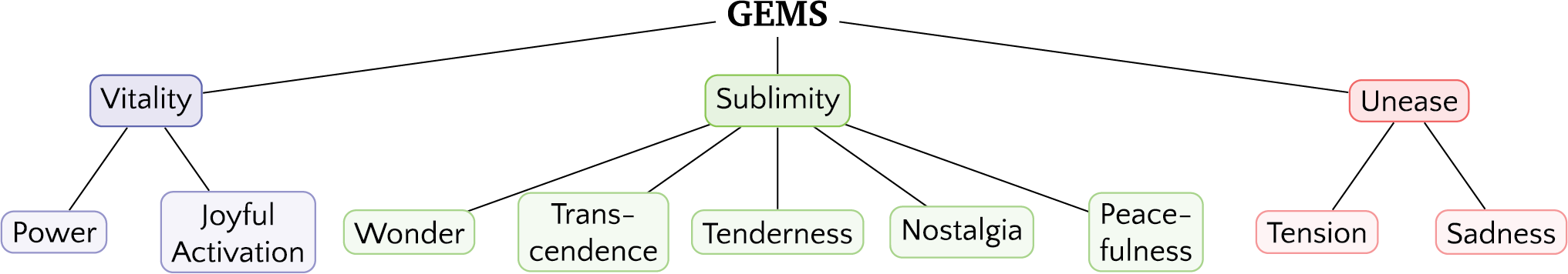
Figure 1
The Geneva Emotion Music Scale with nine dimensions based on the factor analysis in the work of Zentner et al. (2008).
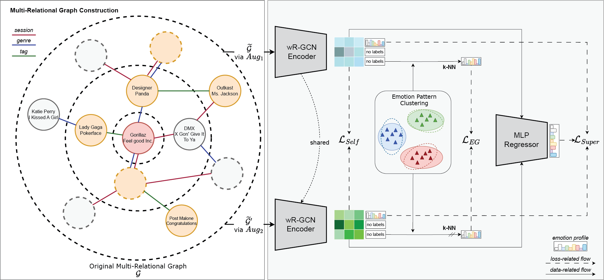
Figure 2
Illustration of SRGNN‑Emo which constructs a multi‑relational graph with nodes representing tracks and edges symbolizing connections based on sessions, genres, or user tags shared among tracks. We used stochastic graph augmentations to generate two distinct graph views, which were processed by a shared encoder to ensure robust and invariant node representations in a self‑supervised manner. Emotion‑guided consistency objective () optimization aimed to align unlabeled nodes with emotion profile patterns of labeled nodes across augmented graph views. The learned node representations were then fed into a multi‑layer perceptron regressor to predict the emotion profile of each track.
Table 1
Multi‑target regression performance for different models across three representation types. The best results are in boldface and the second‑best results are underlined. All improvements of SRGNN‑Emo compared to the second‑best performing model are significant (Wilcoxon signed‑rank test, ). Models marked with † do not use any underlying track representation.
| Rep. | musicnn | MAEST | Jukebox | |||
| Model | RMSE (SE) | (SE) | RMSE (SE) | (SE) | RMSE (SE) | (SE) |
| LR | 0.8443 (0.02) | 0.2470 (0.05) | 1.3821 (0.06) | ‑1.0731 (0.22) | 1.0301 (0.04) | ‑0.1403 (0.09) |
| SVR | 0.8188 (0.01) | 0.2968 (0.01) | 0.7862 (0.01) | 0.3504 (0.02) | 0.9802 (0.02) | 0.0163 (0.01) |
| COREG | 0.8742 (0.02) | 0.1140 (0.05) | 0.8613 (0.02) | 0.1346 (0.08) | 0.8680 (0.02) | 0.1244 (0.05) |
| MLP | 0.8132 (0.02) | 0.3106 (0.02) | 0.8938 (0.03) | 0.1576 (0.08) | 0.8579 (0.02) | 0.2193 (0.06) |
| LP† | 0.9488 (0.03) | 0.0806 (0.01) | 0.9488 (0.03) | 0.0806 (0.01) | 0.9488 (0.03) | 0.0806 (0.01) |
| GCN | 0.8071 (0.02) | 0.3158 (0.04) | 0.7781 (0.02) | 0.3568 (0.05) | 0.7492 (0.04) | 0.4039 (0.05) |
| GAT | 0.8167 (0.03) | 0.2992 (0.07) | 0.7856 (0.02) | 0.3476 (0.05) | 0.7567 (0.02) | 0.3926 (0.03) |
| DGI | 0.8042 (0.02) | 0.3184 (0.06) | (0.01) | 0.3644 (0.06) | (0.02) | (0.04) |
| BGRL | (0.02) | (0.05) | 0.7939 (0.02) | 0.3370 (0.07) | 0.7905 (0.02) | 0.3843 (0.05) |
| MRLGCN | 0.8592 (0.04) | 0.2600 (0.04) | 0.7868 (0.03) | (0.05) | 0.7932 (0.03) | 0.3651 (0.05) |
| DOMR+† | 0.8291 (0.03) | 0.2777 (0.08) | 0.8291 (0.03) | 0.2777 (0.08) | 0.8291 (0.03) | 0.2777 (0.08) |
| SRGNN‑Emo | 0.7973 (0.03) | 0.3305 (0.06) | 0.7707 (0.01) | 0.3724 (0.05) | 0.7411 (0.02) | 0.4180 (0.04) |
Table 2
RMSE scores of models (using the best‑performing representations from Table 1) across multiple emotion targets. Abbreviations of emotion dimensions correspond to wonder, transcendence, tenderness, nostalgia, peacefulness, joyful activation, power, sadness, and tension. All improvements of the best‑performing models (boldface) are statistically significant compared to the second‑best models (underline) per emotion dimension (Wilcoxon signed‑rank test, ).
| Model | wond | tran | tend | nost | peace | joya | power | sadn | tens | GEMS‑9 |
| MLP (musicnn) | 0.9312 | 0.9653 | 0.7330 | 0.8936 | 0.6466 | 0.8099 | 0.8007 | 0.7711 | 0.7675 | 0.8132 |
| DGI (Jukebox) | 0.9059 | 0.9425 | 0.6647 | 0.8094 | 0.7162 | 0.7511 | 0.6627 | 0.6569 | 0.7464 | |
| SRGNN‑Emo (Jukebox) | 0.8972 | 0.9345 | 0.6518 | 0.8026 | 0.6162 | 0.6930 | 0.7425 | 0.7411 | ||
| (A) w/o | 0.9177 | 0.9384 | 0.6532 | 0.8192 | 0.6086 | 0.7050 | 0.7653 | 0.6713 | 0.6829 | 0.7513 |
| (B) w/o | 0.9041 | 0.9387 | 0.6636 | 0.8245 | 0.6110 | 0.7082 | 0.7650 | 0.6845 | 0.6779 | 0.7530 |
| (C) w/o | 1.2372 | 1.0996 | 1.2454 | 1.2210 | 1.3543 | 1.3329 | 1.2424 | 1.2907 | 1.2339 | 1.2508 |

Figure 3
Performance impact of different number of layers in our wR‑GCN component.

Figure 4
Performance impact of different number of emotion profile clusters .

Figure 5
Model performances on different fractions of training data using Jukebox representations.