
Table 1
Details of the nine ragas which are present in our dataset. The 12 notes in the octave (separated by 1 semitone = 100 cents) are denoted by S r R g G m M P d D n N.
| Raga | Tone material |
|---|---|
| Bageshree (Bag) | S R g m P D n |
| Bahar | S R g m P D n N |
| Bilaskhani Todi (Bilas) | S r g m P d n |
| Jaunpuri (Jaun) | S R g m P d n |
| Kedar | S R G m M P D N |
| Marwa | S r G M D N |
| Miyan ki Malhar (MM) | S R g m P D n N |
| Nand | S R G m M P D N |
| Shree | S r G M P d N |
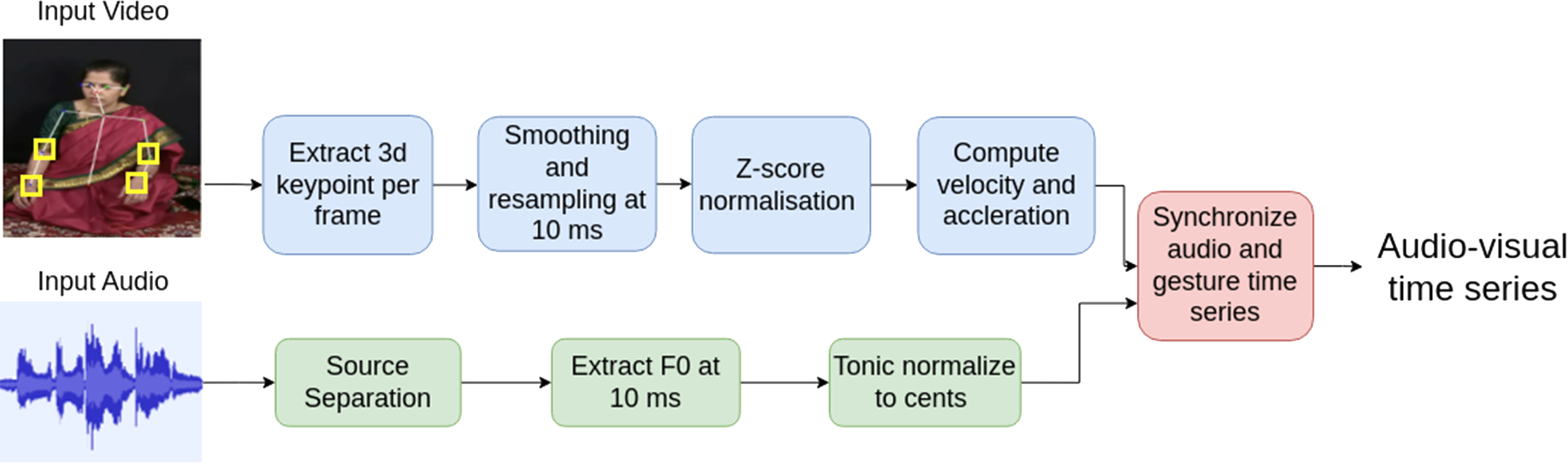
Figure 1
Overall pipeline for preprocessing to get the audiovisual time series. The green path indicates audio processing, the blue path indicates video processing and the red path indicates their combination.

Figure 2
An excerpt from an alap recording of raga Shree performed by the singer AG showing the extracted F0 and right wrist gesture contours. We note a silence (at about 82 s) separating two singing segments.
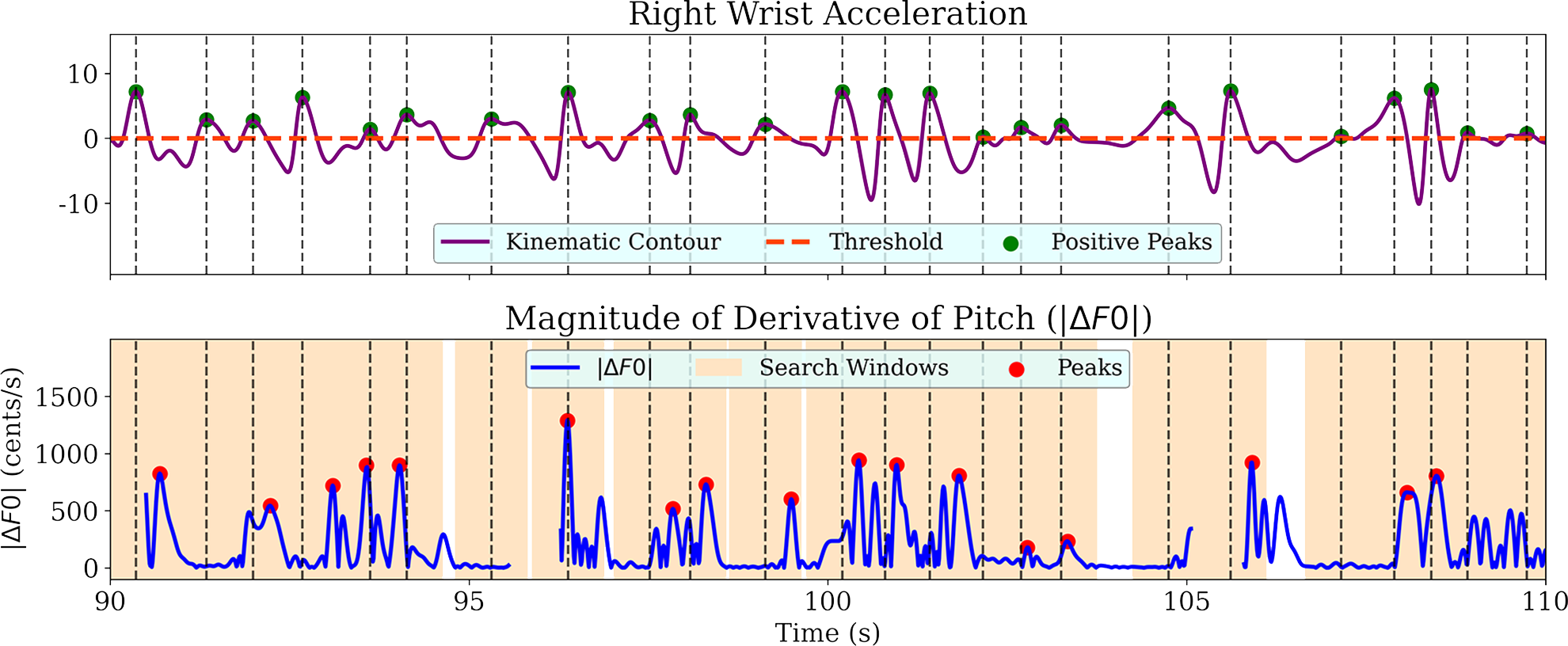
Figure 3
A sample segment from AG_alap1_Bag showing the processing of positive kinematic peaks for the gesture–vocal coupling study. From the gesture contour of right wrist acceleration (top), peaks above the threshold are captured. A window of duration 1 s is taken around the peak location, and the maximum of the contour (bottom) in that window is stored as the corresponding value for the data point in linear regression.
Table 2
Average correlation coefficient between the log of kinematic magnitude trajectory peaks (both positive and negative peaks included; for speed, this is peaks and valleys) and the corresponding peak magnitude of . The reported averages are across the alaps and pakads of each singer for the Vy, S and A of their left (L) and right (R) wrist (W). For the highest coefficient in each row (indicated in bold), p 0.001.
| Singer | RWVy | LWVy | RWS | LWS | RWA | LWA |
|---|---|---|---|---|---|---|
| AG | 0.32 | 0.20 | 0.27 | 0.17 | 0.40 | 0.22 |
| AK | 0.17 | 0.12 | 0.11 | 0.10 | 0.19 | 0.12 |
| AP | 0.06 | 0.15 | 0.02 | 0.12 | 0.09 | 0.12 |
| CC | 0.29 | 0.37 | 0.27 | 0.36 | 0.40 | 0.39 |
| MG | 0.02 | 0.05 | −0.01 | 0.02 | 0.10 | 0.07 |
| MP | 0.08 | 0.15 | 0.05 | 0.16 | 0.09 | 0.19 |
| NM | −0.01 | 0.14 | 0.03 | 0.08 | 0.19 | 0.09 |
| RV | 0.14 | 0.14 | 0.13 | 0.12 | 0.16 | 0.16 |
| SCh | 0.25 | 0.20 | 0.20 | 0.16 | 0.29 | 0.14 |
| SM | 0.08 | 0.16 | 0.03 | 0.09 | 0.12 | 0.18 |
| SS | 0.11 | 0.12 | 0.02 | 0.06 | 0.14 | 0.12 |

Figure 4
A silence‑delimited segment (SDS) with identified stable notes (shaded regions of blue F0 contour) and pitch class distribution (on the left) computed from the entire alap audio with detected svara locations highlighted.
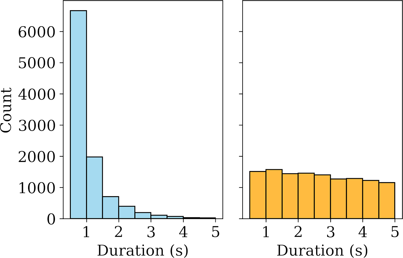
Figure 5
Distributions of duration for stable note (left) and non‑stable segments (right) in our dataset, shown up to a maximum duration of 5 s.
Table 3
The ragas and phrases used in the phrase detection experiment. The svaras S r R g G m M P d D n N correspond to the 12 notes of the Western chromatic scale, with S representing the tonic. The symbols / and \ denote the upward and downward slide, respectively (Rao and van der Meer, 2012; Kulkarni, 2017).
| Raga | Svara (Notes) | Phrase |
|---|---|---|
| Bageshree (Bag) | S R g m P D n | gmD |
| Shree | S r G M P d N | r/P |
| Nand | S R G m M P D N | P\R |
| Miyan ki Malhar (MM) | S R g m P D n N | nDN |
| Bahar | S R g m P D n N | nDN |

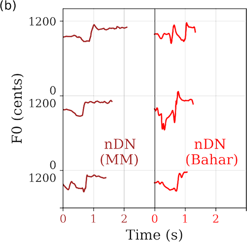
Figure 6
Sample templates for each of the raga characteristic phrases: (a) gmD (purple), r/P (blue) and P\R (violet) and (b) nDN from raga MM (brown) and nDN from raga Bahar (red).
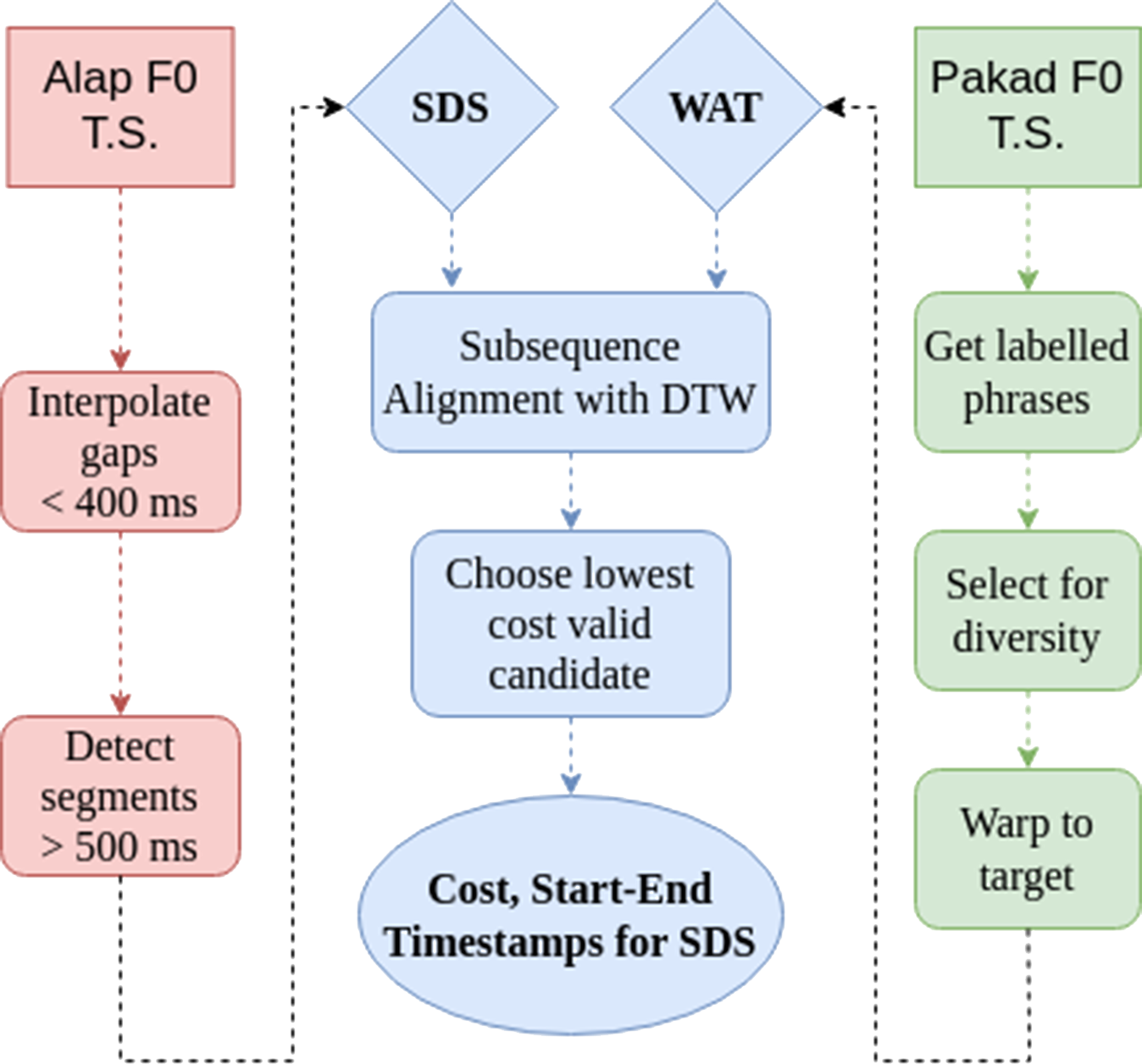
Figure 7
The pipeline for F0‑based segmentation of alap using manually labelled pakad phrases. For warping the pakad phrase templates, a window size of 100 and a penalty of 200 was chosen, while for the subsequence alignment, K = 20 and penalty = 0.1 were chosen (Meert et al., 2016). Segments shorter than 0.5 s were discarded as invalid.

Figure 8
An example of DTW‑based subsequence search of an SDS to identify an instance that best matches the phrase gmD using pakad reference templates. Each of the six warped audio templates is used as a query in the subsequence search, and the query (Q) resulting in the minimum cost is stored. The image on the left shows the audio templates for the phrase gmD. In this example, Q1 is the lowest‑cost query arising from the subsequence alignment shown with respect to the full SDS in the bottom right.

Figure 9
Distribution of the DTW subsequence cost across the SDS of all singer alaps for the best‑matched audio phrase template for P\R of raga Nand. The grey vertical line shows the location of the minimum derived from the kernel density estimate (KDE) fit (dashed red contour), from which the threshold for labelling the SDS as Like and Unlike with reference to the template phrase is derived. This threshold cost marked by the black vertical line is set as half of the location of the minimum of the KDE fit.
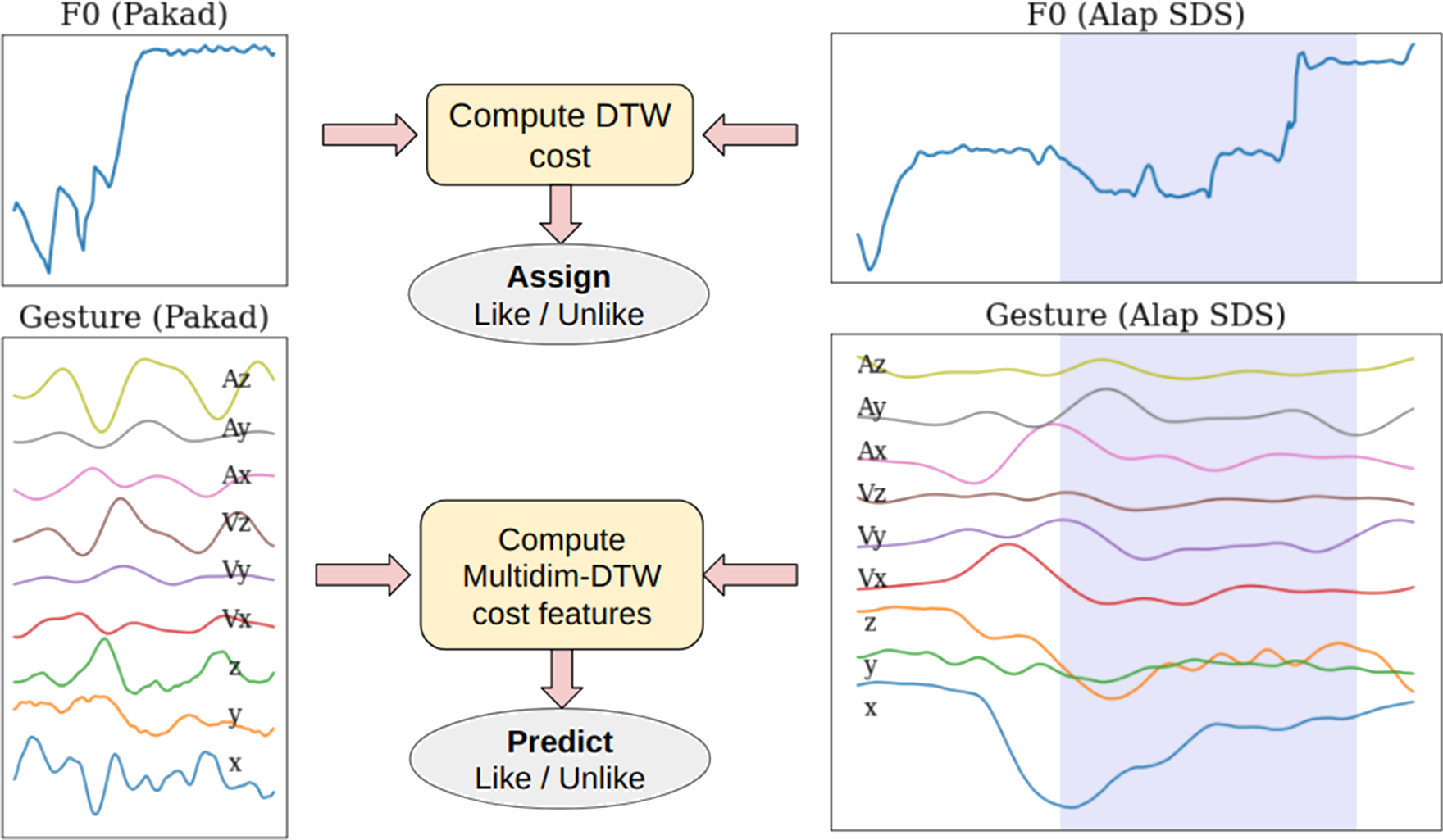
Figure 10
Explaining F0‑based segmentation and labelling (top) to obtain segment boundaries and target labels per SDS for use in the subsequent gesture‑based Like/Unlike prediction task (bottom). The shaded regions on the right represent the SDS subsegment associated with the F0‑based match. The corresponding time‑aligned gesture time series is used to compute the gesture‑based similarity with respect to the pakad (i.e. reference) template time series using multidimensional DTW.

Figure 11
The framework for the evaluation of kinematic features computed from the gesture time series corresponding to stable note and non‑stable segments as detected from the F0 contour.
Table 4
Details of the features used in all variants of the experiment on stable note classification (M, mean; sd, standard deviation; L, left; R, right; W, wrist; E, elbow).
| Abbreviation | Dimensions | Features |
|---|---|---|
| VA‑Mag‑W | 8 | |
| VA‑W | 24 | |
| PVA‑W | 36 | |
| PVA‑E | 36 | |
| PVA‑WE | 72 |

Figure 12
The overall framework for the raga phrase‑based classification. The audio and visual components of a candidate audiovisual (AV) segment (i.e. an SDS from an alap) are separately compared with the respective audio and visual components of a reference phrase segment (from a pakad) to see whether they are together consistent in their estimate of similarity with the reference phrase. We note that the gesture time series (T.S.) is multidimensional, while the audio T.S. is a unidimensional sequence of F0 samples.
Table 5
Singer‑specific counts and F1 scores (%) for stable note detection from segmented gesture time series across the set of instances in the duration range [0.5, 5] s. The segments from all alaps and pakads for each singer are included with the total count provided together with the percentage of segments with stable note labels as obtained from F0‑based labelling. For all the experiment variants, the F1 scores are significantly better than the chance F1 scores (p < 0.001). Bold font indicates the best value per singer.
| AG | AK | AP | CC | MG | MP | NM | RV | SCh | SM | SS | |
|---|---|---|---|---|---|---|---|---|---|---|---|
| Total count | 1778 | 2146 | 2485 | 2965 | 1928 | 2252 | 1846 | 1720 | 973 | 2328 | 2064 |
| Percentage of stable notes (%) | 53.8 | 45.3 | 47.5 | 35.3 | 57.4 | 56.2 | 40.0 | 39.6 | 52.8 | 45.8 | 31.3 |
| VA‑Mag‑W | 80.3 | 77.5 | 75.2 | 71.5 | 80.7 | 81.2 | 75.4 | 69.7 | 83.2 | 76.6 | 61.7 |
| VA‑W | 91.3 | 87.9 | 85.2 | 83.7 | 87.7 | 86.1 | 88.1 | 80.3 | 91.2 | 82.8 | 74.4 |
| PVA‑W | 92.9 | 90.4 | 87.1 | 84.5 | 90.1 | 89.1 | 90.3 | 84.9 | 94.0 | 85.9 | 76.4 |
| PVA‑E | 91.6 | 86.5 | 85.3 | 82.5 | 86.8 | 86.9 | 84.5 | 80.6 | 89.7 | 84.6 | 71.2 |
| PVA‑WE | 93.7 | 90.5 | 89.8 | 85.4 | 91.3 | 89.6 | 89.7 | 84.9 | 93.8 | 88.1 | 77.3 |
Table 6
F1 scores (%) for the different stable‑note‑detection experiments. The “singer specific” score indicates the count‑weighted average of F1 scores for PVA‑WE in Table 5. Next, we carry out cross‑validation in three different types: uniform split (10‑fold CV), unseen singer split (11‑fold CV) and unseen raga split (9‑fold CV). The features PVA‑WE were used in all cases. The total number of segments classified is 22,485 (all alaps and pakads across all 11 singers and nine ragas), with the percentage of stable notes at 45.3%.
| Singer‑specific | Uniform split | Unseen raga | Unseen singer | |
|---|---|---|---|---|
| Folds (#) | 10 | 10 | 9 | 11 |
| F1 (%) | 88.2 | 86.1 | 84.4 | 80.5 |
Table 7
F1 scores (%) for motif detection for each of the raga phrases computed with the uniform‑singer splits in 10‑fold CV across the different DTW cost feature vector choices. The final two rows pertain to the prediction of the first‑mentioned raga’s phrase when the test set contains the pooled instances of both ragas. The best performance in each row is in bold font. The * indicates the value is statistically significant () when compared with a chance classifier which predicts ‘Like’ with a probability equal to the percentage of like segments..
| Phrase | Raga | #SDS | Count | Like (%) | DTW‑D (1) | DTW‑I (1) | DTW‑LR (2) | DTW‑Ind (36) | DTW‑Ind‑W (18) |
|---|---|---|---|---|---|---|---|---|---|
| r/P | Shree | 505 | 415 | 50.1 | 69.0* | 70.5* | 64.7* | 65.9* | 66.4* |
| gmD | Bageshree | 489 | 331 | 53.2 | 59.9 | 65.4* | 65.1* | 64.6* | 65.2* |
| PR | Nand | 435 | 301 | 45.9 | 30.5 | 22.9 | 66.4* | 74.6* | 75.8* |
| nDN | MM | 429 | 155 | 54.2 | 77.3* | 77.3* | 66.8* | 79.3* | 71.4* |
| nDN | Bahar | 433 | 257 | 48.6 | 68.9* | 67.4* | 54.8 | 71.8* | 74.3* |
| nDN | MM, Bahar | 862 | 396 | 21.2 | 2.4 | 4.6 | 54.3* | 52.1* | 44.6* |
| nDN | Bahar, MM | 862 | 438 | 28.5 | 15.0 | 1.6 | 46.4* | 46.4* | 43.1* |
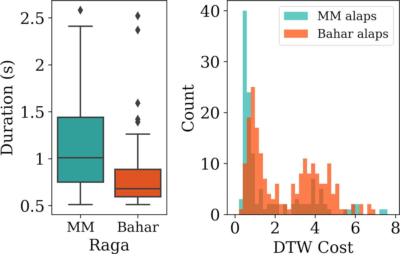
Figure 13
Left: Comparing the duration distributions of the ‘Like’ instances for the ragas MM and Bahar. Right: Histogram of DTW costs (across each of the MM and Bahar alaps) for the F0‑contour subsequence search with respect to reference templates of phrase nDN from pakads of raga Miyan ki Malhar (MM).
Table 8
F1‑scores for the detection of raga Shree r/P with unseen‑singer splits (i.e. leaving one singer out of CV) across the different DTW cost feature vectors. Bold fonts indicate the highest obtained performance for each singer.
| AG | AK | AP | CC | MG | MP | NM | RV | SCh | SM | SS | |
|---|---|---|---|---|---|---|---|---|---|---|---|
| Count | 31 | 38 | 41 | 52 | 28 | 27 | 30 | 47 | 36 | 36 | 49 |
| Like (%) | 71 | 57.9 | 43.9 | 30.8 | 50 | 48.1 | 56.7 | 61.7 | 38.9 | 61.1 | 42.9 |
| DTW‑D (1) | 82.6 | 60.4 | 68.3 | 56.1 | 64.7 | 77.4 | 68.3 | 76.5 | 68.3 | 78.4 | 60.0 |
| DTW‑I (1) | 83.7 | 56.0 | 74.4 | 56.1 | 68.6 | 81.3 | 68.3 | 75 | 68.3 | 80.9 | 60 |
| DTW‑LR (2) | 50.0 | 64.0 | 81.1 | 40.8 | 58.3 | 42.1 | 68.8 | 61.8 | 77.8 | 76.2 | 59.7 |
| DTW‑Ind (36) | 62.9 | 62.8 | 76.9 | 48.8 | 61.5 | 63.6 | 64.5 | 56.0 | 76.5 | 74.4 | 62.5 |
| DTW‑Ind‑W (18) | 66.7 | 59.6 | 75 | 55.3 | 64.5 | 57.1 | 70.6 | 51.1 | 85.7 | 77.3 | 63.8 |
Table 9
F1‑scores for the detection of raga Shree r/P with singer‑specific splits (i.e. 10‑fold CV entirely within the individual singer’s data set) across the different DTW cost feature vectors. Bold fonts indicate the highest obtained performance for each singer.
| AG | AK | AP | CC | MG | MP | NM | RV | SCh | SM | SS | |
|---|---|---|---|---|---|---|---|---|---|---|---|
| Count | 31 | 38 | 41 | 52 | 28 | 27 | 30 | 47 | 36 | 36 | 49 |
| Like (%) | 71 | 57.9 | 43.9 | 30.8 | 50 | 48.1 | 56.7 | 61.7 | 38.9 | 61.1 | 42.9 |
| DTW‑D (1) | 83 | 71.2 | 0 | 11.8 | 80.0 | 48.3 | 74.4 | 76.3 | 81.5 | 75.9 | 0 |
| DTW‑I (1) | 88.0 | 73.3 | 0 | 40.0 | 59.3 | 23.5 | 73.7 | 76.3 | 63.6 | 75.9 | 0 |
| DTW‑LR (2) | 76 | 71.2 | 48 | 43.5 | 76.9 | 43.5 | 72.2 | 76.3 | 92.3 | 75 | 58.8 |
| DTW‑Ind (36) | 81 | 78.0 | 77.8 | 85.7 | 82.8 | 69.6 | 82.4 | 74.6 | 85.7 | 74.4 | 66.7 |
| DTW‑Ind‑W (18) | 87.0 | 60.5 | 77.8 | 78.6 | 75.9 | 64 | 74.3 | 73.3 | 89.7 | 78.3 | 42.9 |
Table 10
F1 scores (%), aggregated across the 11 singers, for the detection of the phrase r/P under each of the listed train–test split conditions. Results are presented for two DTW cost feature vector choices.
| Singer‑specific | Uniform split | Unseen singer | |
|---|---|---|---|
| Folds (#) | 10 | 10 | 11 |
| DTW‑Ind (36) | 77.9 | 65.9 | 63.9 |
| DTW‑LR (2) | 65.7 | 64.7 | 61.8 |