
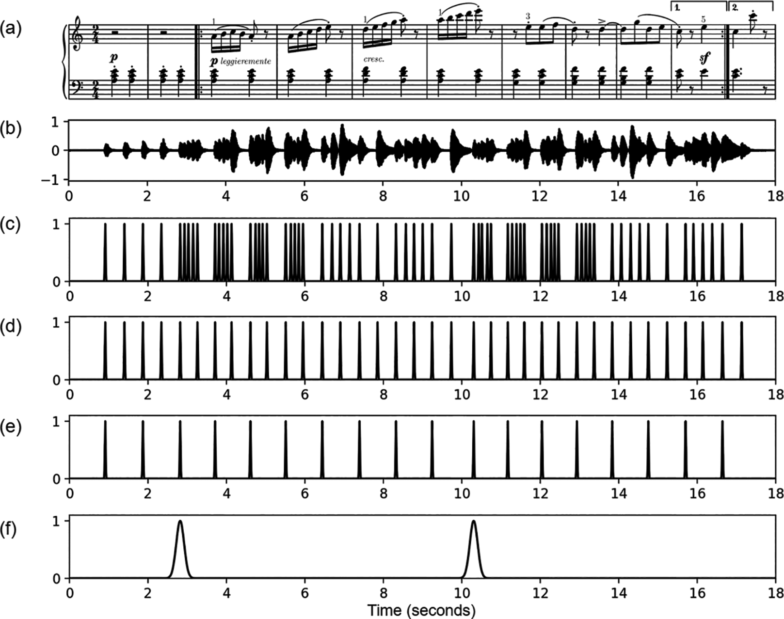
Figure 1
Idealized novelty functions for various MIR tasks. (a) Musical score of the beginning of the second piano etude from Op. 100 by Burgmüller. (b) Audio recording of the corresponding excerpt. (c) Onset detection. (d) Beat tracking. (e) Downbeat (measure) tracking. (f) Boundary estimation for music structure analysis.
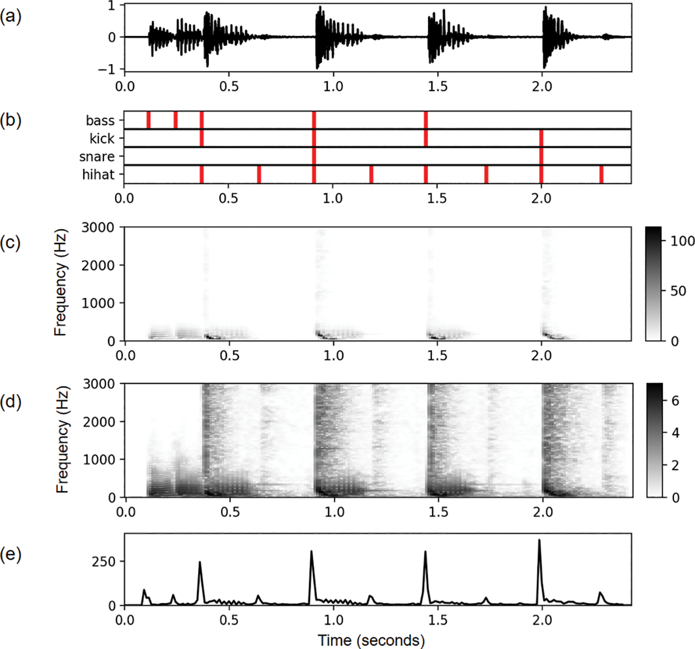
Figure 2
Computation of a novelty function based on spectral flux used for onset detection. The music excerpt corresponds to the beginning of the song “Another One Bites the Dust” by Queen. (a) Music signal (shown as waveform). (b) Annotation of target onsets for the applicable instruments. (c) Magnitude spectrogram. (d) Compressed magnitude spectrogram. (e) Novelty function.
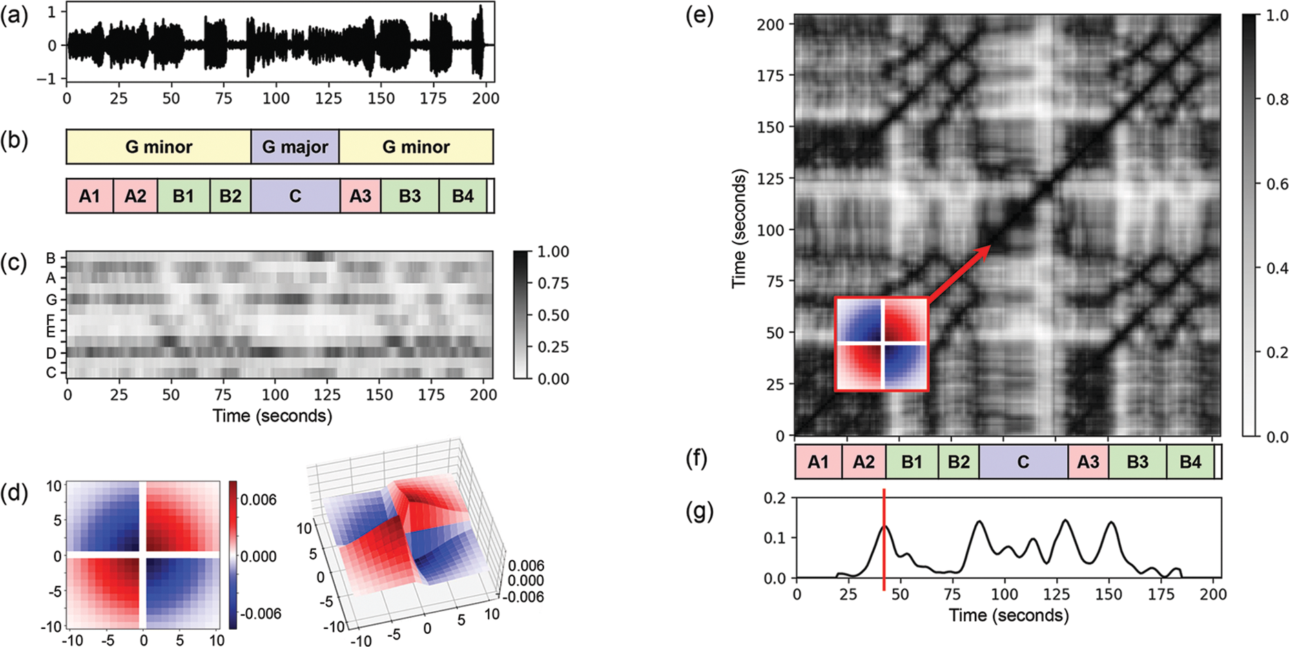
Figure 3
Novelty‑based boundary detection for music structure analysis. The example is based on a recording of the “Hungarian Dance No. 5” by Johannes Brahms. (a) Music signal (shown as waveform). (b) Annotation of local key segments and the musical form. (c) Chromagram. (d) Checkerboard kernel shown as 2‑dimensional and 3‑dimensional plot. (e) Self‑similarity matrix with kernel shifted along the main diagonal. (f) Annotation of the musical form. (g) Novelty function with a vertical line indicating the position of the kernel shown in (e).
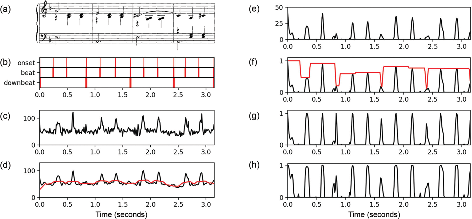
Figure 4
Enhancement strategies. The example is based on an audio excerpt (orchestral version) from Dimitri Shostakovich’s “Waltz No. 2, Suite for Variety Orchestra No. 1.” (a) Musical score of piano‑reduced version. (b) Annotations of onset, beat, and downbeat positions. (c) Novelty function based on spectral flux (see Figure 2). (d) Smoothed novelty function and local average function (red curve). (e) Enhanced novelty function . (f) Max‑normalized novelty function and local max function (red curve). (g) Novelty function after local‑max normalization. (h) Novelty function from (f) after applying the hyperbolic tangent function.
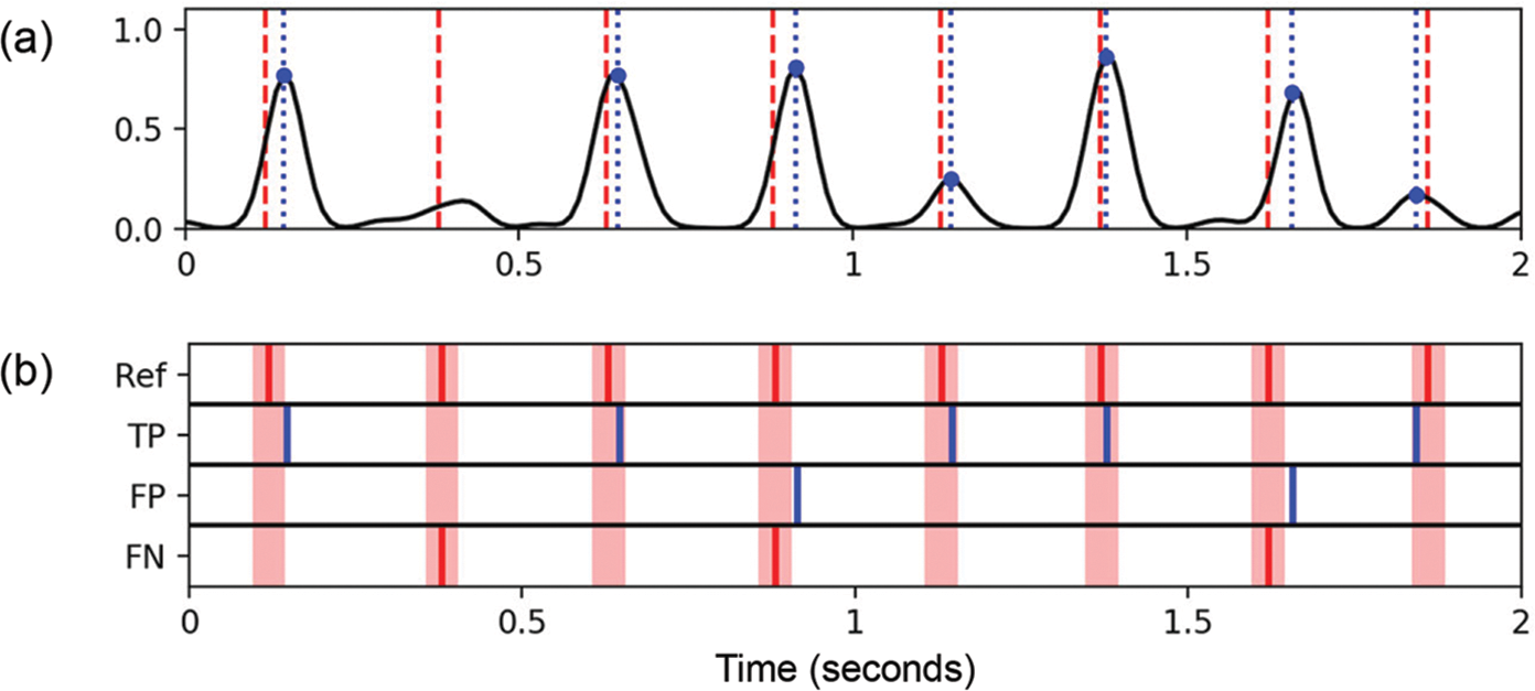
Figure 5
Illustration of precision, recall, and F‑measure with error tolerance. (a) Novelty function with estimated positions (blue dotted lines) and reference positions (red dashed lines). (b) Illustration of reference positions (Ref), true positives (TP), false positives (FP), and false negatives (FN), with error tolerance (indicated by red‑shaded regions). One has #TP , #FP = 2, and #FN , thus yielding , and .
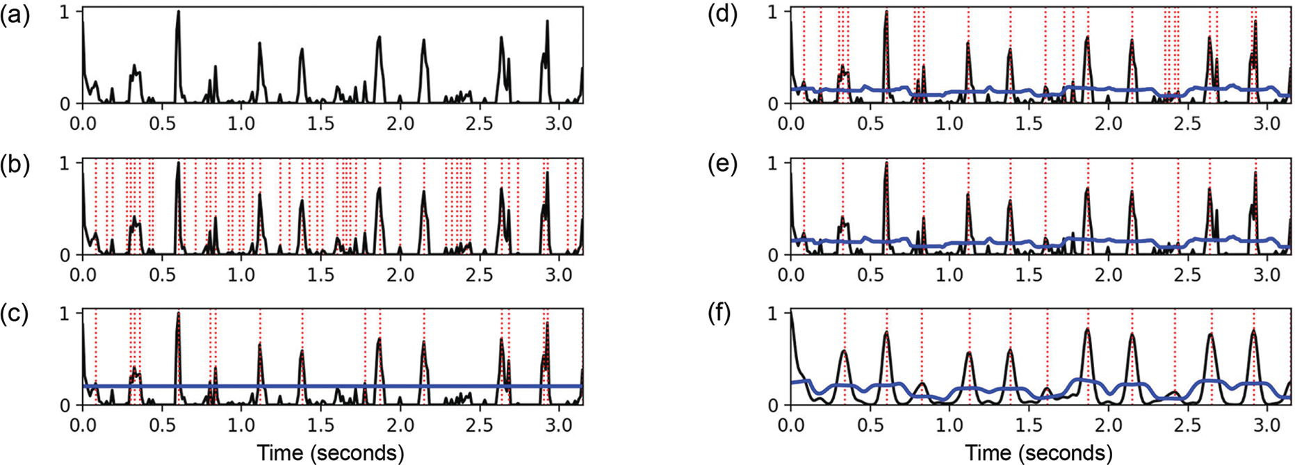
Figure 6
Illustration of peak picking based on different heuristics. (a) Novelty function. (b) Simple peak picking (selected peak positions are indicated by red vertical lines). (c) Usage of a global threshold (shown as a blue horizontal line). (d) Usage of a local threshold (shown as a blue curve). (e) Usage of an additional distance constraint. (f) Application of Gaussian smoothing, max normalization, and a local threshold.
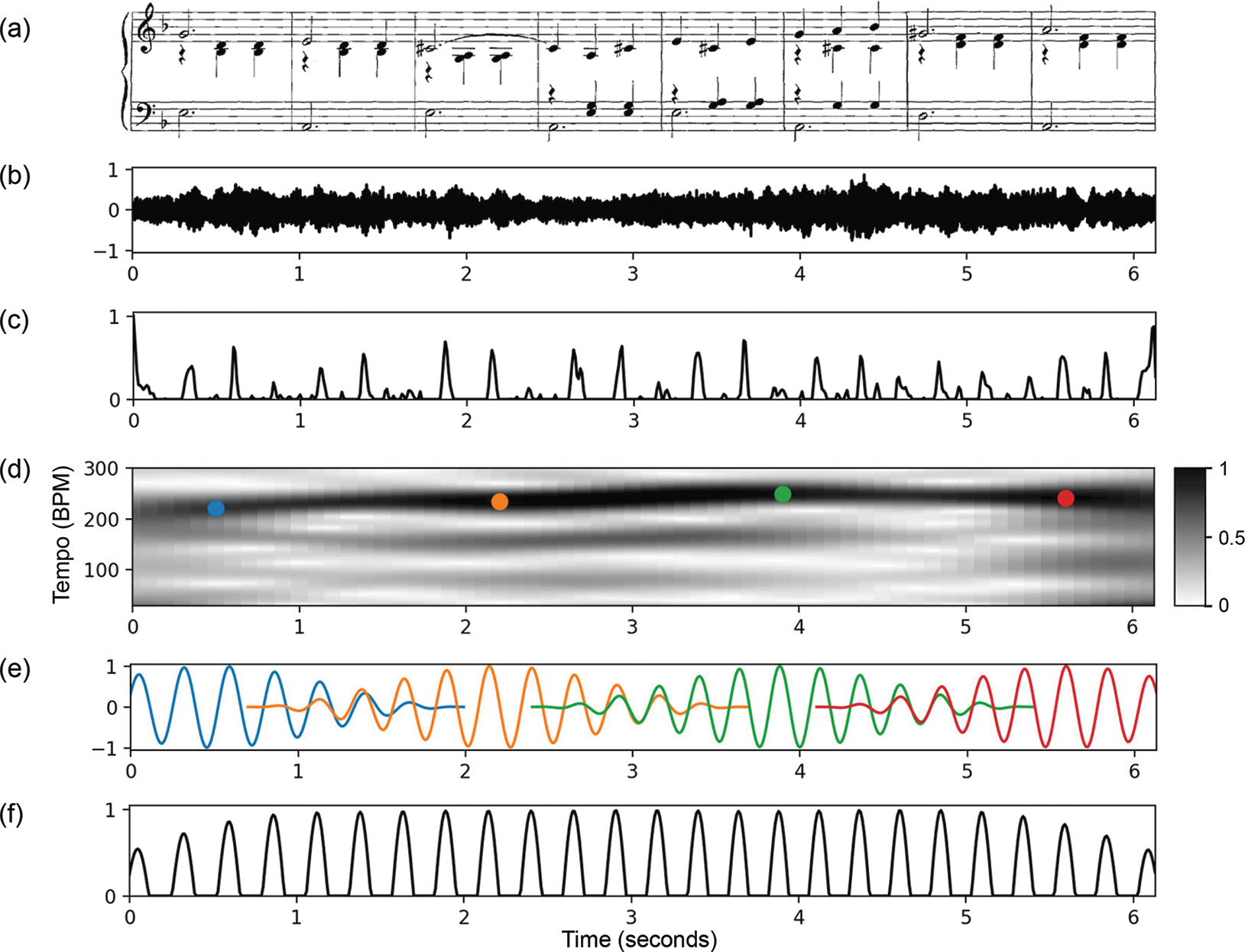
Figure 7
Illustration of the computational pipeline for deriving the predominant local pulse (PLP) function, continuing the Shostakovich example introduced in Figure 4, (a) Musical score of piano‑reduced version. (b) Audio recording of the corresponding excerpt. (c) Novelty function. (d) Tempogram showing timedependent tempo maxima, indicated by colored dots. These dots are displayed at only four selected time positions for better visibility. (e) Optimal windowed sinusoids corresponding to the maxima. (f) PLP function obtained by applying overlap‑add and half‑wave rectification techniques.