
1 Introduction
Music Information Retrieval (MIR) plays a key role in analyzing and understanding musical content, with beat tracking standing out as a central task within this field. The general idea of beat tracking is to have a system that analyzes music and automatically taps along with the beat, similar to what human listeners would do (Dixon and Cambouropoulos, 2000; Ellis, 2007). The human perception of beats in music can occur at different metric levels, for example, the tactus level (quarter notes), the measure level (bars), and the tatum level (temporal atom), which refers to the fastest repeating temporal pattern in the music (Müller, 2021).
Besides beat tracking, there are several closely related concepts: While tapping and marking beat positions in a piece of music, beats can be counted and grouped into bars, a process called meter tracking (Holzapfel and Grill, 2016; Klapuri et al., 2006). Identifying the first beat of each bar is helpful for many music applications and is referred to as downbeat tracking (Böck et al., 2016b; Durand et al., 2015; Krebs et al., 2016). Analyzing the number of beats per minute (BPM) helps to identify the tempo of the music, which is commonly known as tempo tracking (Krebs et al., 2015).
In this work, we mainly focus on the task of beat tracking that involves identifying the time positions of beats within a music recording and is essential for MIR applications ranging from music transcription to rhythm-based interactive systems. Typically, beat tracking is a two-step process: first, calculating an activation function to extract frame-wise beat likelihood from the music signal, and second, performing a postprocessing method to determine final beat positions from the activation function.
Most existing beat tracking methods are designed for offline use and rely on access to the entire music track for processing. In recent years, deep learning has led to substantial improvements in beat tracking with approaches such as Temporal Convolutional Networks (TCN) (Böck and Davies, 2020; Davies and Böck, 2019), Transformer (Zhao et al., 2022), or SpecTNT-TCN (Hung et al., 2022). With the growing demand for real-time applications like interactive music systems and live performance tools, the need for online-capable beat tracking algorithms has become more evident. This trend is reflected in contributions such as BeatNet (Heydari et al., 2021), Novel-1D (Heydari et al., 2022), or the most recent model BEAST-1 (Chang and Su, 2024).
When employing online approaches for real-time applications or integrating them into larger interactive systems, two prominent challenges emerge: latency and controllability. First, latency encompasses delays not only from the beat tracker itself but also from network communication, audio output processing, or controller input lags. These delays make it challenging to maintain synchronization between analyzed input audio streams and generated output audio streams. Second, controllability in this context refers to the challenges most online beat trackers face in being easily adjustable for specific real-time application requirements. Most real-time beat tracking systems lack explicit control over parameters such as pulse level (e.g., quarter-note or eighth-note level) or the amount of latency.
In this article, we present a real-time beat tracking system built on the predominant local pulse (PLP) concept (Grosche and Müller, 2011), originally developed for offline use. Our main contribution is the successful transformation of the PLP-based algorithm into a real-time procedure. With our approach, we achieve beat detection performance comparable to that of most other online beat trackers. In contrast to previous beat trackers, our method allows for achieving zero latency while remaining lightweight and easily controllable. In particular, our approach incorporates beat lookahead functionality to mitigate latency effects in interactive real-time systems and provides enhanced controllability through adjustable parameters.
To evaluate the influence of the lookahead feature on beat detection performance, we conduct experiments using a variety of datasets. In addition to quantitative evaluation, we demonstrate the practical usability of our system through two real-world applications for interactive music making and educational music gaming. These applications creatively utilize the output of our system, highlighting its controllability and versatility. In summary, our real-time beat tracking system represents a lightweight algorithm that is especially useful for interactive music software development. By bridging the gap between offline beat tracking methods and real-time application requirements, our system opens up new possibilities for musicians to use real-time beat tracking for their interactive music systems.
The subsequent sections of this article follow this structure: In Section 2, we explore the original PLP-based algorithm. Section 3 discusses the conversion of this algorithm into a real-time procedure. In Section 4, we analyze the system output resulting from this real-time procedure. With Section 5, we conduct multiple experiments, and their results are discussed in Section 6. We demonstrate our real-time system through two real-world scenario applications in Section 7. Finally, Section 8 concludes our method. Additional materials and audio examples are available on a supplemental website.1
2 PLP-Based Algorithm
Before discussing how to convert the PLP-based algorithm into a real-time procedure (Section 3), we first look at the original offline procedure (Grosche and Müller, 2011). All the essential steps for calculating the PLP are illustrated in Figure 1 (left column).
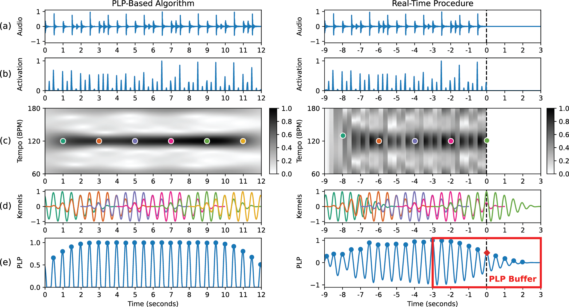
Figure 1
Illustration of the original offline PLP-based algorithm (left side), as described in Section 2, and the real-time procedure (right side), detailed in Section 3. (a) Audio signal. (b) Activation function. (c) Tempogram. (d) Pulse kernels. (e) PLP function. To provide clearer visualization and illustrate the general idea, we plot kernels only at 2-second intervals.
First, the audio signal (Figure 1a) is transformed into an activation2 function for time positions . The peaks of the activation function (Figure 1b) indicate the likelihood of observing a beat at time positions . To identify local periodic patterns, we perform a Short-Time Fourier Transform (STFT) on . For this, we define a window function for that is normalized and centered around each time position , resulting in a total window size of . For an arbitrary but fixed time position , the window defines a neighborhood indexed by . The complex-valued Fourier coefficient
obtained from the STFT is defined for time positions , frequencies , and local time indices . From the Fourier coefficient , we derive a Fourier tempogram , given by
This time–frequency representation of the activation function , as illustrated in Figure 1c, is commonly measured in BPM rather than Hertz, with a tempo parameter . Utilizing the Fourier tempogram relies on two assumptions commonly employed in beat tracking. First, beat positions go along with note onsets, and, second, beat positions are periodically spaced. These assumptions are exploited by comparing local sections of the activation function with windowed sinusoidal kernels , given by the equation
for , as shown in Figure 1d. To obtain a local beat (or pulse) tracker, we choose for each time position a kernel that optimally matches the local tempo structure of the signal within a given tempo range , as illustrated with colored dots in Figure 1c. For instance, when denoting , we refer to a tempo range spanning from 30 to 240 BPM. In Equation 3, is defined as the tempo parameter that maximizes the tempogram for each time position .
Additionally, represents the phase of the windowed sinusoid with tempo that best correlates with the local section around of the activation function .
To obtain a globally defined pulse tracker, the final step of the original offline procedure involves overlap-adding all optimal pulse kernels over time to form a global pulse function :
This curve, which reveals predominant local pulse (PLP) information, is referred to as the PLP curve. To reach its final state, the PLP function undergoes two additional computation steps, included in Equation 6: normalization and half-wave rectification. The constant
ensures the normalization of the PLP function, keeping the values within the range of . With halfwave rectification, we only consider the positive values of the PLP function, where for a non-negative real number and for a negative number . For a more detailed description, we refer to Grosche and Müller (2011).
3 Real-Time Procedure
MIR is an area of research that often deals with the analysis of entire corpora. The algorithms used for these analyses typically operate offline. In contrast to this, the algorithms used for real-time analysis face multiple challenges. This includes working with causal data only, addressing the trade-off between accuracy and latency, and meeting audio processing deadlines, as discussed by Stefani and Turchet (2022). In adapting our model from offline to real-time (Section 3.1), we encountered three significant differences, which we discuss in more detail in the following subsections. First, data is streamed in small blocks, requiring the balancing of latency and computation times (Section 3.2). Second, only causal data is available, affecting the overall accuracy of the beat tracker (Section 3.3). Third, data needs to be stored in buffers, enabling access to previous time frames for handling larger context windows (Section 3.4).
3.1 Real-Time PLP algorithm
The original offline procedure outlined in Section 2 can be transformed into a real-time procedure, as depicted in Figure 1 (right column). Given the centric nature of the kernels around each time position , the kernel window is essentially divided into two halves, see Figure 1d. The left half of the kernel window supporting is utilized to compute the pulse structure based on past and present data, while the right half supporting (] is used to extrapolate this pulse structure to future time positions. This allows the superimposed kernels to predict future beat positions, as illustrated in Figure 1e.
To describe the real-time procedure, we update the equations in Section 2 as follows. Let denote the current time position, where we have access to activation values for all time positions . The complex- valued Fourier coefficient from Equation 1 becomes
which is defined for all time positions , frequencies , and local time indices . For the current time position , we obtain a real-time PLP function called
which is defined for all time positions and has access to all kernels for . For normalization, we use the constant from Equation 7, which ensures that the values lie within the range of . Additionally, for the real-time PLP function, we choose to skip half-wave rectification and preserve a more sinusoidal state to better capture dynamic pulse changes over time. Note that the kernels are computed based on (Equation 8), denoted with for the Fourier tempogram (Equation 2), for the tempo parameter (Equation 4), and for the phase (Equation 5). The PLP buffer, depicted in Figure 1e, displays only the section of for , containing all the necessary information to compute the subsequent time position . Note that for this buffer, our perspective shifts from a linear time scale to a centric viewpoint, where the center of the buffer represents the current time position (which corresponds to the physical buffer time position , as illustrated in Figure 2).
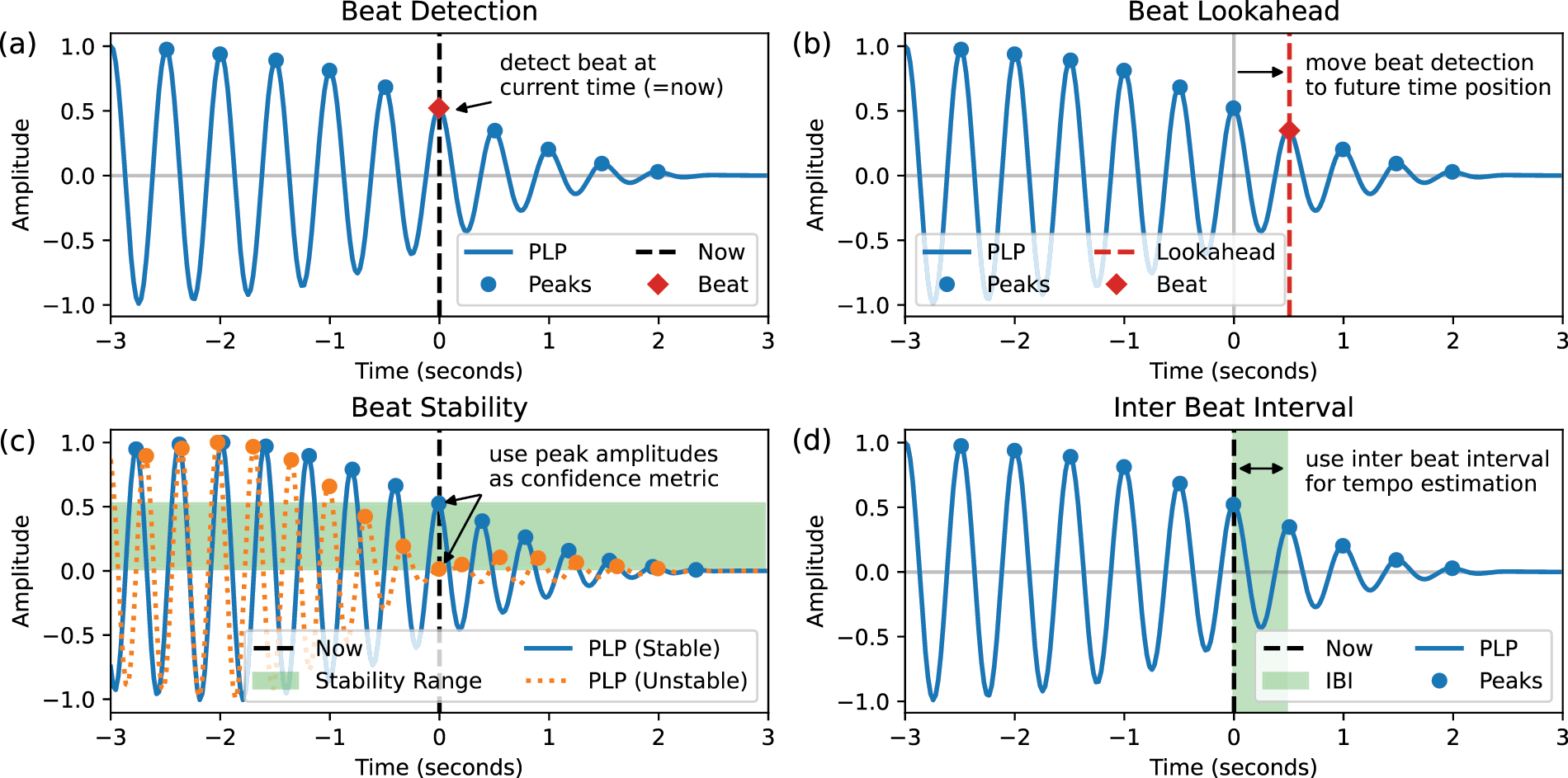
Figure 2
The output of the real-time beat tracking system: (a) Beat Detection (Section 4.1). (b) Beat Lookahead (Section 4.3). (c) Beat Stability (Section 4.4). (d) Inter Beat Interval (Section 4.5).
3.2 Audio streaming
The main difference between offline and real-time processing lies in how data is delivered. In offline processing, the entire audio track is available at any time. Conversely, in real-time processing, audio data is streamed continuously as it becomes accessible. Streamed audio is commonly processed in small blocks of data known as frames, which directly correspond to the time positions introduced in Section 2. Each frame contains a fixed frame size of recent audio data sampled at a fixed audio sampling rate . The duration of a single frame is called frame period T, as given by the equation
Consequently, when we receive a frame of data, we are inherently operating with a latency equivalent to one frame period . For example, if a real-time system runs with an audio sampling rate and a frame size samples, the system latency based on the frame period is . Reducing the frame size to minimize system latency is often not feasible because the frame period also determines the available computation time per frame.
3.3 Causal data processing
PLP operates with centric kernels , analyzing a specific time position within a larger context window by utilizing both past and future data, with local time indices . However, for the real-time procedure, only causal data is available, limiting the indices to . While delaying the computation to await future data is possible, this approach is not feasible for real-time applications. For this reason, in our real-time model, we only utilize past and present data for PLP computation. This helps avoid additional latency but also impacts other aspects of the beat tracking pipeline, as we will discuss in the following.
The tempogram is based on only past and present activation data, which has multiple effects. First, the data for calculation is essentially half the size and therefore less accurate. Second, the lack of future data makes it harder to adapt to upcoming tempo changes. Third, the activation data displays a discontinuity, abruptly dropping to zero due to the absence of future data. This discontinuity introduces artifacts, manifesting as vertical lines in the tempogram, as depicted in Figure 1c.
The real-time PLP function incorporates only past and present kernels , as we restrict the kernel summation in Equation 9 to local time indices . Consequently, the right half of the PLP buffer, which represents future pulse data, consistently exhibits a falling slope due to the absence of overlapping kernels on that side of the buffer. This leads to less prominent peaks in the PLP buffer for characterized by overall lower amplitude values, as illustrated in Figure 1e.
3.4 Data buffering
Compared to a single frame size , the kernel window for PLP is relatively long, typically utilizing kernel sizes of s. Therefore, a single frame of audio data is insufficient for computing PLP, and it is necessary to collect and store frames in a buffer. To achieve this in a memory-efficient manner, we buffer only as much data as necessary to compute the current frame. For this purpose, a First-In-First-Out circular buffer is utilized, where the oldest values are dropped as new values are added. For real-time PLP, there are two computations where buffers are needed. First, to compute a kernel, an activation buffer with half kernel size is required , supporting . Second, to overlap-add kernels with previous kernels, a PLP buffer with full kernel size is needed (), supporting . The PLP buffer is fully described by for the section in Equation 9.
4 System Output
The primary objective of the real-time procedure (Section 3) is to update the PLP buffer with every new frame of data, thereby generating all the system output, as we will discuss in the following subsections.
4.1 Beat detection
With Figure 2a, we demonstrate the process of beat detection in our real-time beat tracking system. For offline processing, the goal of beat detection is to compile a list of beat positions, indicating when beats occur relative to the start of an audio track. For real-time audio streaming, the objective of beat detection is to determine if a beat should be triggered at the current time position . This is achieved by analyzing the current state of the PLP buffer and using a simple peak picking method to identify peak positions within the section . If a peak falls at the center time position of the PLP buffer (), a beat occurs at the current time position and should be triggered immediately.
4.2 Beat context
Even though the beat detection method outlined in Section 4.1 primarily focuses on the center time position of the PLP buffer, every peak provides additional valuable information. They create a form of beat context around the current time position , giving insights into both past and potential future beat positions. This functionality proves useful for real-time applications, as demonstrated in Section 7.2. The extent to which past and future information is available can be adjusted by modifying the PLP kernel size . However, this also affects how sensitive the beat tracker is to tempo variations in the music: Increasing the kernel size reduces the tracker’s sensitivity to tempo fluctuations. Conversely, decreasing the kernel size enhances the tracker’s responsiveness to tempo changes.
4.3 Beat lookahead
For beat detection, as discussed in Section 4.1, we typically use the center position of the PLP buffer as the “decision line.” However, by considering the beat context (Section 4.2), we can shift this decision line to any time position , including future time positions , as illustrated in Figure 2b. To achieve this, we introduce the beat lookahead, an input parameter influencing the real-time beat tracking system’s behavior. Instead of detecting beats at the center time position of the PLP buffer, the beat lookahead defines an offset, to move the decision line by a fixed number of frames to detect and trigger beats ahead of time.
Although triggering beats earlier may not appear intuitive, it becomes a valuable solution in addressing significant latency issues inherent in most real-time applications. These delays often arise from various sources, including audio processing, network communication, or input controller lags. Therefore, the beat lookahead is crucial for compensating for these latencies and ensuring synchronization between the analyzed input signal and the generated output signal.
However, predicting beats ahead of time comes with a trade-off: the accuracy of beat detection diminishes to some extent, which we elaborate on in Section 6.4.
4.4 Beat stability
Every time beat detection (Section 4.1) occurs, the PLP function can have varying amplitude values for peak positions , which directly fall at the decision line, such as the center time position of the PLP buffer . These amplitude values serve as indicators of beat stability, as depicted in Figure 2c. A high peak amplitude signifies a stable beat situation, indicating that the neighboring optimal kernels were similar in tempo and constructively added up over time (constructive interference). Conversely, a low peak amplitude indicates an unstable beat situation, where neighboring optimal kernels with different tempi have canceled each other out (destructive interference). To this end, beat stability values can be utilized to control parameters in real-time applications, such as the volume of an accompaniment track, as detailed in Section 7.1.
Between the minimum and maximum peak amplitudes lies an entire stability range. Since the PLP function is normalized (see constant from Equation 7), the beat stability can have values between . In this way, the peak amplitudes act as a confidence metric that can be used in addition to beat detection. For example, if an application requires consistent beat output sequences without unstable and noisy beat sections, a stability threshold can be introduced. This threshold can serve as an optional beat filter that allows beats to be processed only when they surpass a certain amplitude value, as we will discuss in Section 7.2.
4.5 Inter beat interval and local tempo
Providing a local tempo measure for the current time position is particularly beneficial for interactive music making (Section 7.1), where the tempo can serve as an input parameter for time-based music instruments and effects plugins (e.g., sampler, reverb, delay, or echo). With PLP, we have two different approaches for determining local tempo. First, on the frame level, the PLP kernel is calculated based on the tempo parameter , which directly yields a local tempo value. Second, the PLP function offers a more consistent tempo measure, defined by the inter beat interval of two consecutive peaks, as illustrated in Figure 2d.
The tempo output can be bounded by setting minimum and maximum tempo values for the PLP procedure, thereby defining a specific tempo range . Modifying this tempo range allows us to influence the pulse level at which the beat tracker should operate, such as the normal tactus level (quarter notes) or one tempo octave higher with double tactus level (eighth notes). For instance, if the expected tempo for a beat tracking application is around 100 BPM, we can focus the tempo output on the range for normal tempo or choose to force double tempo output.
5 Experiments
To evaluate the described methods, we carry out multiple experiments. First, we compare our method with various low-latency beat trackers under specific oracle conditions and against methods from the existing literature for beat performance, latency, and tempo range. With the second experiment, we concentrate on an assessment of context-sensitive beat evaluation on different tempo ranges. Third, we evaluate our real-time procedure across different kernel sizes. Last, in the fourth experiment, we investigate the impact of the lookahead parameter on beat detection performance.
5.1 Datasets
For our experiments, we employ a diverse set of commonly used datasets. We report on the average track duration, tempo, and stability in Table 1. To calculate tempo stability, we convert all inter beat intervals to tempo values and normalize them by dividing each by its respective average track tempo, maintaining a tolerance interval of for stable tempi. For a formal definition of tempo stability, we refer to Schreiber et al. (2020).
Table 1
Overview of the datasets used for evaluation.
| Dataset | Dataset (Total) | Track (Average) | ||||
|---|---|---|---|---|---|---|
| Name | Tracks | Length | Type | Duration | Tempo | Stability |
| Ballroom | 698 | 6h 03m | Excerpt | |||
| GTZAN | 993 | 8h 16m | Excerpt | |||
| Rock | 200 | 12h 53m | Full | |||
| RWCPop | 100 | 6h 46m | Full | |||
The Ballroom dataset, introduced by Gouyon et al. (2006), provides audio excerpts categorized by different dance music styles, displaying a wide variety of tempo ranges. GTZAN, described by Tzanetakis and Cook (2002), comprises audio excerpts spanning a diverse range of genres, including Country, Metal, Hiphop, Reggae, Jazz, and Classical. The Rock dataset, as introduced by Clercq and Temperley (2011), features songs listed in Rolling Stone magazine’s “500 Greatest Songs of All Time” and generally exhibits lower overall tempo stability compared to the other datasets. Additionally, the RWCPop dataset, described by Goto et al. (2002), provides a collection of pop songs with full audio recordings and high tempo stability.
Figure 3 offers an overview of the datasets, showing that Rock and particularly GTZAN include tempo values exceeding the range handled by our online model, see also Section 5.5. Given that online models typically function within a more limited tempo spectrum compared to offline models, it is important to note that the wider tempo span of these datasets could potentially affect the overall performance of beat estimation.
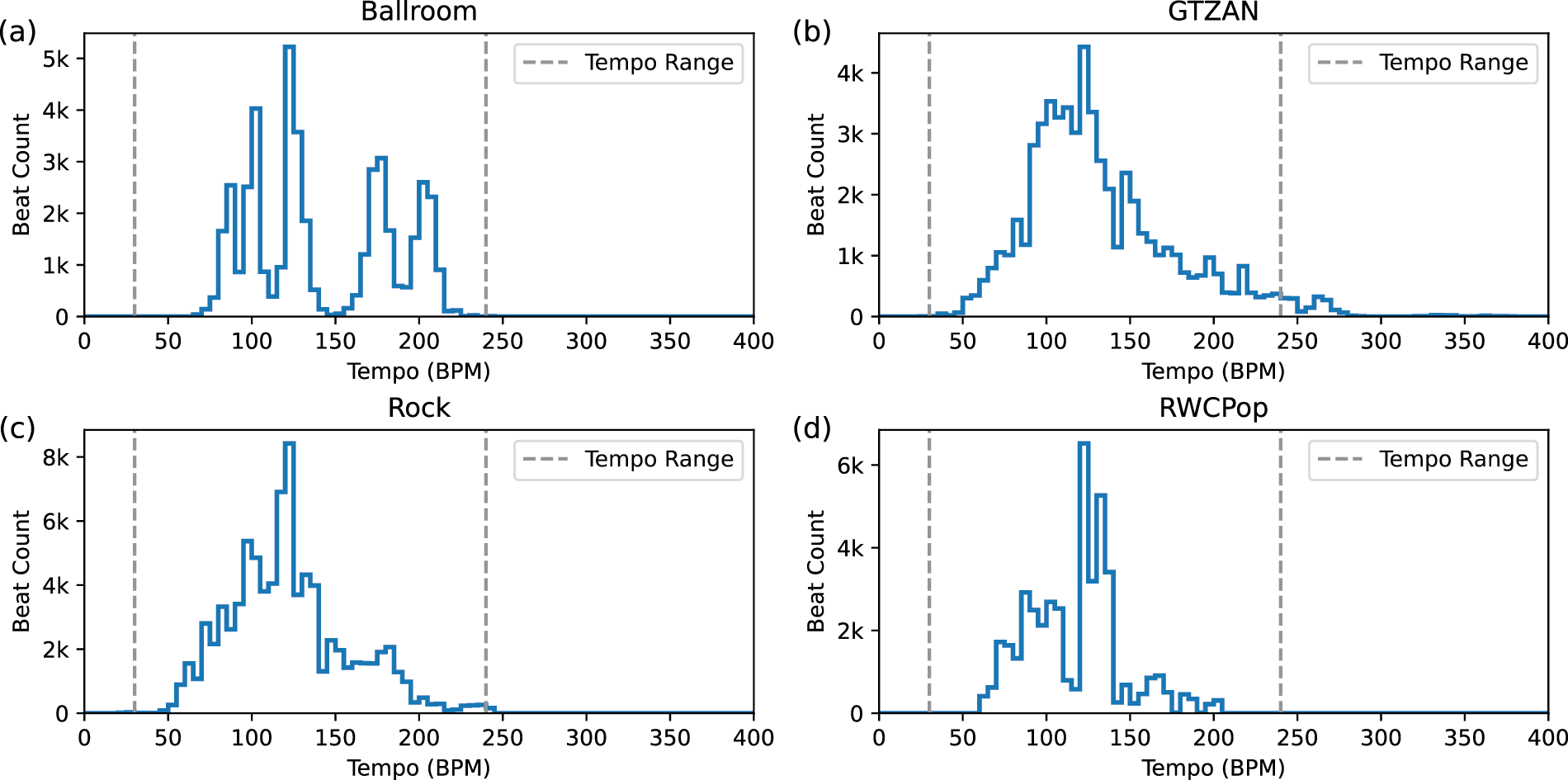
Figure 3
Beat-wise distribution of inter beat intervals (IBI) in various datasets, considering a tempo resolution bin size of 5 BPM. The tempo range for our online model (30–240 BPM) is indicated with dashed lines.
5.2 Activation functions
For the activation functions, we explored two distinct online methods. The first method (RNN) involves a machine learning approach, utilizing an online Recurrent Neural Network (RNN) activation with a specifically chosen single Long Short-Term Memory (LSTM) model (Böck and Schedl, 2011). In particular, we adopted the approach utilizing madmom’s RNNBeatProcessor (online=True) along with their pre-trained LSTM model 4 (Böck et al., 2016a). It is worth noting that these LSTM models are trained on the Ballroom dataset and therefore may exhibit superior performance on it compared to other datasets. The second method (GT) is a “ground truth” activation, which is derived from annotated beat positions. For each time position , it outputs an amplitude value of 1 at annotated beat positions and 0 otherwise. To achieve this, we convert annotated beat positions (in seconds) into frame indices based on the frame period (see Equation 10). This approach is valuable for analyzing post-processing methods independently of the activation, assuming best possible activation performance.
5.3 Post-Processing methods
In this paper, the term “post-processing” is used for a beat tracking method that determines beat positions from an activation function. Specifically, our PLP-based post-processor takes an activation function as input, generates the PLP pulses as described in Section 2, and detects the beats accordingly. For our experiments, we outline the following post-processing methods: As a baseline reference, labeled as PLP-Off, we use the original PLP concept to directly compare the transition from offline to online. Our online adaptation of the original PLP method is referred to as PLP-On.
5.4 Evaluation measures
For evaluating beat estimation, we employ the standard F1-score metric with a tolerance window of ms, as implemented in mir_eval (Raffel et al., 2014). For context-sensitive evaluation, we apply the L-correct metric, as introduced by Grosche and Müller (2011). With this evaluation method, we consider not just a single beat but a series of consecutive estimated beats, each with a temporal context of length . This is similar to how a listener would tap along to music, often needing a sequence of beats to adapt to tempo changes. Therefore, context-sensitive evaluation is valuable for evaluating how well our method can handle larger beat contexts (Section 4.2). To avoid initialization artifacts in the evaluation, we disregard all beats occurring before 5 s of each music track.
5.5 Experiment setup
For our experiments, we focus on an application-ready setup, using an audio sampling rate and a frame size samples. These configurations are typical for real-time audio hardware, such as an audio interface, resulting in a frame period ms. The default tempo range for our experiments is , unless stated otherwise. With a tempo of 30 BPM, the beat events are 2 s apart, which can be considered as approaching the lower bound of human tempo perception. With an upper tempo of 240 BPM, we cover a full range of three tempo octaves (doubling the tempo of 30 BPM for three times). With TR40, we denote a tempo range of of the average track tempo, assuming that the mean tempo of a music recording is given. Throughout this paper, we consistently use the PLP method with a fixed kernel size of 6 s for all experiments and examples. Further discussion on this choice is provided in Section 6.3.
6 Results and Discussion
6.1 Overview and methods comparison
In Table 2, we compare various beat tracking methods for F1-score, latency, and tempo range to assess the performance of our models on the GTZAN dataset. The latency values listed are based on the individual frame period of each respective method (see Equation 10). Our default online model RNN-PLP-On uses the RNN activation as input for the PLP-On post-processing and achieves an F1-score of , which falls within the range of most other online beat trackers. However, our approach has only a very small latency of 11.61 ms. The leading online model in our list, BEAST-1, achieves an F1-score of , but it comes with a significantly higher latency of 46.44 ms. This delay could be perceived as distinct acoustic events by human ears, making it unsuitable for certain real-time audio applications where precise synchronization between input and output audio streams is important. Furthermore, we introduce RNN-PLP-On-Zero with an F1-score of , which stands out as the only model in the table with a latency of 0 ms. Zero latency is achieved by offsetting the frame period (see RNN-PLP-On) with a lookahead of 1 frame, allowing beats to be triggered 11.61 ms ahead of time. With RNN-PLP-On-TR40 and GT-PLP-On, we showcase potential enhancements of our online model when utilizing oracle conditions, such as a known average tempo range (TR40) or a perfect ground truth activation function (GT). In addition, we report on offline PLP models RNN-PLP-Off, providing a more comprehensive comparison between offline to online processing.
Table 2
Comparing various low-latency online beat trackers under specific conditions (C1, . . . , C5) and against existing literature for beat performance, latency, and tempo range, utilizing the GTZAN dataset. A tempo range of of the average track tempo is denoted by TR40 and ground truth activation by GT.
| Model | Mode | Comments | F1-score (%) | Latency (ms) | Tempo (BPM) |
|---|---|---|---|---|---|
| RNN-PLP-On | Online | our model | 74.72 | 11.61 | 30 - 240 |
| RNN-PLP-On-Zero | Online | our model (zero latency) | 74.68 | 0.00 | 30 - 240 |
| Exploratory Studies: Oracle Conditions | |||||
| RNN-PLP-On-TR40 | Online | (C1) use avg. track tempo | 75.11 | 11.61 | track (mean) |
| GT-PLP-On | Online | (C2) use GT activation | 91.93 | 11.61 | 30 - 240 |
| RNN-PLP-Off | Offline | (C3) use non-causal data | 79.07 | – | 30 - 240 |
| RNN-PLP-Off-TR40 | Offline | (C4) use avg. track tempo | 82.00 | – | track (mean) |
| GT-PLP-Off | Offline | (C5) use GT activation | 97.83 | – | 30 - 240 |
| Methods Overview: Comparing with Literature | |||||
| BEAST-1 | Online | Chang and Su (2024) | 80.04 | 46.44 | 55 - 215 |
| Novel-1D | Online | Heydari et al. (2022) | 76.48 | 20.00 | 55 - 215 |
| BeatNet | Online | Heydari et al. (2021) | 75.44 | 20.00 | 55 - 215 |
| Böck-FF | Online | Böck et al. (2014) | 74.18 | 46.44 | 55 - 215 |
| SpecTNT-TCN | Offline | Hung et al. (2022) | 88.7 | – | – |
| Transformer | Offline | Zhao et al. (2022) | 88.5 | – | – |
| TCN | Offline | Böck and Davies (2020) | 88.5 | – | – |
6.2 Context-Sensitive evaluation on tempo range
With Figure 4 we report on results using the context-sensitive L-correct metric for different tempo ranges. When analyzing our online model PLP-On with the activation function RNN, we observe a decrease in F1-score from (no context) to (). This reflects the fact that detecting a series of beats accurately is more challenging than detecting a single beat. Further increasing the number of consecutive beats from to , the F1-scores remain almost constant, with a slight decrease of about (from to ). This implies that the PLP method is inherently designed to effectively handle larger beat contexts, a characteristic that holds true for the online method as well.
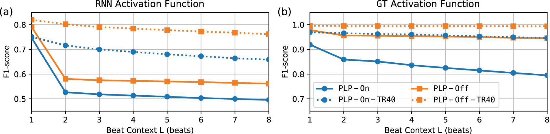
Figure 4
F1-score and L-correct metric for different activation functions and various post-processing methods on the GTZAN dataset. A tempo range of average track tempo is denoted by TR40.
When analyzing RNN-PLP-On-TR40, which utilizes a tempo range of of the average track tempo, we notice a much smaller decrease in F1-score from (no context) to . Furthermore, for all other consecutive beats from to , the F1-scores remain consistently higher compared to RNN-PLP-On, with only a slight decrease of approximately (from to ). Similarly, for the activation functions GT depicted in Figure 4b, we observe consistent F1-scores, particularly evident for the tempo range TR40. This suggests that a notable improvement in context-sensitive beat performance can be achieved if the average tempo of the analyzed music is known and utilized for specific beat tracking tasks, thus highlighting the tempo range as a valuable hyperparameter for controlling real-time applications.
6.3 Kernel size evaluation
In Figure 5, we assess our real-time procedure across various kernel sizes. Considering the best possible activation function GT in Figure 5b, we observe consistent behavior across all datasets. When the kernel size is above 6 s, the F1-score remains stable; however, when it falls below 6 s, the F1-score starts to drop significantly. Based on this observation, we opted to fix the kernel size at 6 s for our experiments, aiming to find a balance between stability in beat estimation and responsiveness to tempo changes in the music. A more realistic scenario is depicted with the activation function RNN in Figure 5a. In this case, we observe minimal variation in F1-score across different kernel sizes across various datasets. The F1-score begins to decrease only when the kernel sizes fall below 3 s. This suggests that our real-time procedure can effectively accommodate a wide range of kernel sizes, enabling adjustment of the beat context with minimal impact on F1-score.
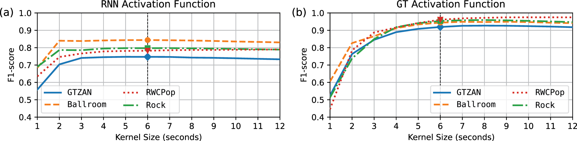
Figure 5
F1-score for different kernel sizes of PLP-On across various activation functions on different datasets.
6.4 Lookahead impact analysis
We now discuss the impact of the lookahead parameter on the beat detection performance and start with Figure 6a, focusing on RNN and GTZAN as an example. The corresponding data is reported in Table 3. For a lookahead of 0 frames (0 ms), the F1-score is at , which we already reported for RNN-PLP-On in Table 2. Using a lookahead of 1 frame (11.6 ms), there is only a small difference in F1-score for a total of . Using a 10-frame lookahead (116.1 ms) results in , which is useful for compensating network and processing delays, as demonstrated in Section 7.1. With 50 frames (580.5 ms), comparable to the inter beat interval size (500 ms) at 120 BPM, the F1-score drops to . At 100 frames (1161.0 ms), the F1-score falls to , and at 200 frames (2322.0 ms), it declines significantly to . Overall, the impact of lookahead on the F1-score is relatively small, especially for values below 50 frames (580.5 ms), emphasizing its importance as a valuable parameter for controlling and compensating latency in real-time beat tracking systems.
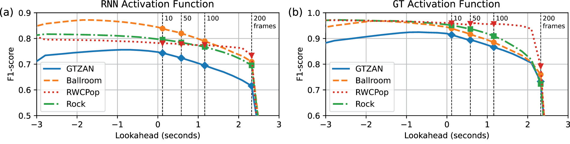
Figure 6
F1-score of various settings for lookahead of PLP-On for various activation functions across different datasets, see Table 3 for numbers.
Table 3
The F1-score of lookahead settings in frames (and milliseconds) of PLP-On for different activation functions across different datasets, with each F1-score accompanied by the difference (in parenthesis) to the zero lookahead.
| Settings | F1-score (%) vs. Lookahead | ||||||
|---|---|---|---|---|---|---|---|
| Lookahead in frames (ms) | 0 (0.0) | 1 (11.6) | 10 (116.1) | 50 (580.5) | 100 (1161.0) | 200 (2322.0) | |
| RNN | GTZAN | 74.72 | |||||
| Ballroom | 84.39 | ||||||
| RWCPop | 78.22 | ||||||
| Rock | 79.74 | ||||||
| GT | GTZAN | 91.93 | |||||
| Ballroom | 94.44 | ||||||
| RWCPop | 96.10 | ||||||
| Rock | 95.39 | ||||||
Comparing different datasets for lookahead performance, we observe a correlation with the tempo deviation of each dataset (see Table 1), which indicates the level of tempo variation across all songs. The dataset RWCPop exhibits the highest stability () and the lowest tempo deviation ( BPM) among the datasets analyzed, experiencing the smallest drop in F1-score () at 200 frames lookahead. In contrast, at 200 frames lookahead, Rock ( BPM), GTZAN ( BPM), and Ballroom ( BPM) experience drops in F1-score of , , and respectively. This suggests that lookahead can be employed with minor impact on beat detection performance, particularly for highly stable music genres such as Pop. This is particularly evident in the case of GT, Figure 6b, where the RWCPop dataset demonstrates stable F1-scores for up to 2 s of lookahead, distinguishing itself from other datasets.
Note that all datasets in Figure 6 show higher F1-scores for negative lookahead (adding latency to make a more accurate decision by waiting for future data). However, since our focus is more on compensating for latency rather than adding latency for real-time applications, we do not discuss this fact any further.
7 Applications
In this section, we present two application prototypes for interactive music making (Section 7.1) and educational music gaming (Section 7.2) that utilize the system output of our real-time beat tracker in a creative way.
7.1 Interactive music making
We start off with a demo for interactive music making, closely following the work by Meier et al. (2021). The terminal application, named “Beat Command Line Interface” (beatcli.py), is implemented in Python and built upon the real-time procedure detailed in Section 3.
With Figure 7, we show a block diagram of the application. It accepts input arguments (A) to select a device/channel of the audio input (B) and configure various parameters required for the audio analysis (C). It continuously executes a complete PLP real-time procedure and uses data buffering (Section 3.4) to update the PLP model for every new frame of audio provided by the input audio streaming (Section 3.2). Upon beat detection (Section 4.1) within the current time frame, both terminal output (D) and network output (E) with corresponding local pulse information are provided, as shown in Figure 9. This system output (Section 4) can be received by software clients (F), such as a Digital Audio Workstation (DAW), or hardware devices (G), such as microcontrollers, to utilize the transmitted local pulse information.
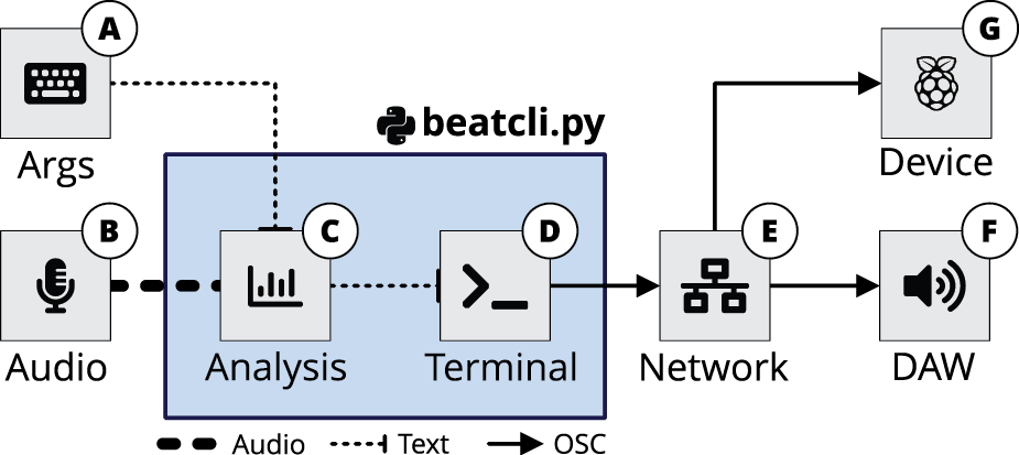
Figure 7
A block diagram of the beatcli.py terminal application. (A) Input arguments. (B) Audio input. (C) Audio analysis. (D) Terminal output. (E) Network output. (F) Receiving software. (G) Receiving hardware.
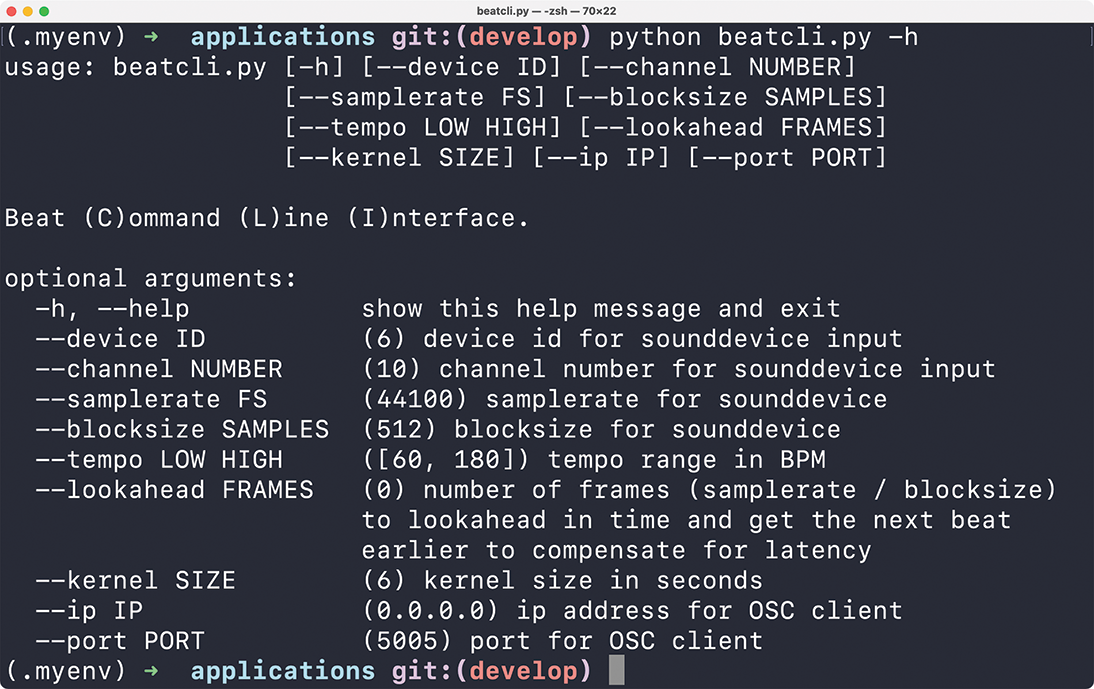
Figure 8
The help function of the beatcli.py application with information about input arguments.
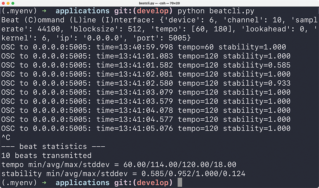
Figure 9
The terminal output of the beatcli.py application showing the system in action.
The help function of beatcli.py (Figure 8) offers detailed explanations of the input arguments. The real-time audio streaming (Section 3.2) relies on the Python module sounddevice,3 which receives the first four arguments to specify the desired hardware. The next three arguments control the settings of the beat tracker, including the tempo range in BPM to set the pulse level, the lookahead (Section 4.3) in FRAMES to compensate for latency, and the kernel SIZE in seconds to determine the beat context (Section 4.2). Last, two arguments configure the network output. beatcli.py serves as an Open Sound Control (OSC) server, sending pulse information over the network to a client with a specified IP address and PORT number.
With Figure 9, we illustrate the terminal output of beatcli.py, detailing the transmitted pulse information. Upon application launch, an overview of default settings is provided. Below this follows a table of detected beats, each row containing columns with local pulse information. Initially, the IP address and PORT of the OSC message being sent out are displayed. Subsequently, a time value provides a timestamp of when the beat detection (Section 4.1) occurred. Following this, a tempo value indicates the local tempo computed from the inter beat interval (Section 4.5). Finally, a value for beat stability (Section 4.4) is displayed. A value of 1.0 represents a beat with a steady tempo and maximum stability, while values close to zero signify a relatively unstable tempo and beat structure.
To demonstrate a real-world use case of the application, we describe a real-time accompaniment system using beatcli.py. Suppose we are playing an instrument and intend to utilize our beat tracker to trigger samples in a DAW synchronized with the beat of our music. The stability parameter allows us to control the volume, ensuring that samples are only audible when beats are stable. With every beat we update the global tempo of the DAW, thereby adjusting the playback speed of the samples to match the tempo of our playing. With the tempo range settings, we can limit the beat triggers to certain tempo octaves, accommodating different tempo variations such as normal, or double tempo. The kernel size parameter allows us to adjust the overall beat context, making the tracker either more stable or more responsive to tempo changes. Finally, the lookahead value enables us to fine-tune the system to compensate for any noticeable network and processing delays, ensuring that the playback feels natural and not lagged.
7.2 Educational music gaming
In this section, we introduced an application for educational music gaming, closely following the work by Meier et al. (2022).
We present a prototype jump-and-run game named “Rock Your Beats,” which is illustrated in Figure 10. The player’s goal is to tap along in sync with the beat of the music, by pressing a button on a touch screen, keyboard, or gaming controller. In doing so, the player must aim to hit moving “beat creatures” with a dropping rock positioned at the center of the game world. Each beat creature represents one beat, and one point is awarded for each hit.
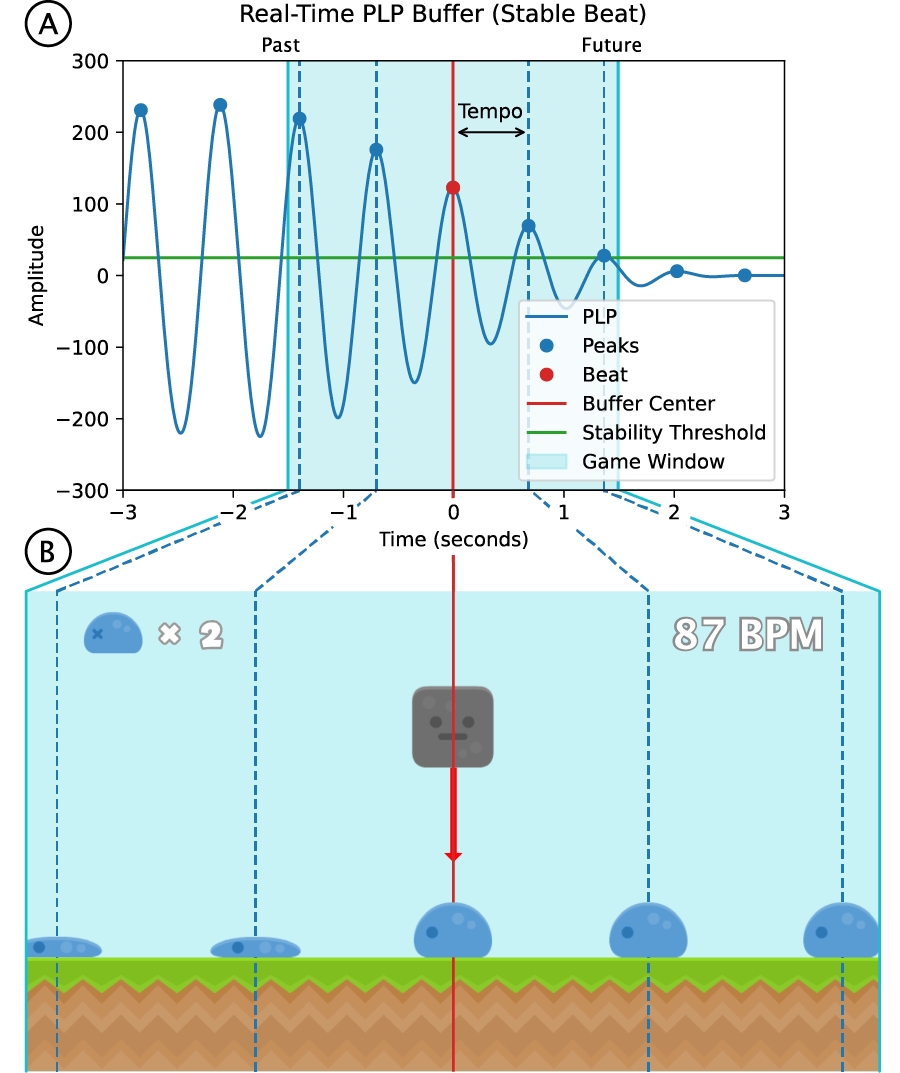
Figure 10
The educational music game “Rock Your Beats” (bottom) with the corresponding real-time PLP buffer (top), used to derive the positions of “beat creatures” in the game world.
The game world is generated in real-time from music in the player’s environment by using the streamed audio (Section 3.2) of a microphone input signal. The center of the game world (the rock) represents the current point in time and thus relates to the center of the PLP buffer (at second zero), as discussed in Section 3.3. The beat creatures are placed at the peak positions of the PLP curve, using the beat context (Section 4.2). Therefore, the beat creatures follow the same movement from the right (future) to the left (past) positions as the peaks of the PLP curve and cross the central player position in sync with the beat of the music, as discussed in Section 4.1. If no stable beat structure is detected in the input signal, the peaks of the PLP curve have a rather low amplitude, as explained in Section 4.4. If this amplitude is below a certain stability threshold, no beat creatures are created in the game world, to avoid unpredictable and noisy beat illustrations. As a consequence, beat creatures only appear if music with a stable beat is played. The time range that is visually represented in the game, the game window, is closely related to the beat context (Section 4.2). In this way, the game window can also be chosen smaller to avoid the visualization of inaccurate beat predictions in the distant future and to determine how much visual support the player gets. The inter beat interval (Section 4.5) can be used to display the current local tempo in the game. Finally, with the beat lookahead (Section 4.3), the game can be adjusted to compensate for latency that might occur with the game visualization and controller input delays. For a more detailed discussion of this gaming application, we refer to Meier et al. (2022).
8 Conclusions
In this paper, we introduced a real-time beat tracking system designed to deliver zero latency and enhanced controllability for interactive music applications. In addition to beat detection, our model generates valuable supplementary outputs, including beat context, beat stability, and inter beat interval analysis for local tempo estimation. Leveraging the beat lookahead technique, our method effectively compensates for latency by up to several hundred milliseconds in real-time audio systems. Furthermore, our model demonstrates enhanced controllability, allowing real-time applications to adjust latency compensation, pulse level, and beat context. This versatility proves particularly beneficial for real-time beat tracking tasks, where maintaining synchronization between the analyzed input audio stream and the produced output audio stream is crucial, thereby preventing any noticeable delay in audio perception. We validated and tested the capability of our model through experiments and two real-world scenario applications focused on interactive music making and educational music gaming. As a result, our model serves as a practical and lightweight tool for musicians to fine-tune their real-time audio setups and achieve the desired latency perception, while also opening up new creative controllability for real-time beat tracking applications.
For future research, our goals include conducting additional experiments, such as evaluating the lookahead feature of our model on smaller tolerance windows and investigating beat performance on more challenging datasets. Additionally, we aim to enhance our real-time pipeline by integrating newly developed beat activation models into our post-processing method as they become available in the future. Recognizing the practical utility of our system, we are committed to continuing the development of interactive applications and demonstrations. Specifically, we plan to create a real-time beat tracking audio plugin to enable musicians to use our method for studio mixing or interactions live on stage.
Acknowledgements
We thank the anonymous reviewers and the section editor for their helpful and constructive comments. The International Audio Laboratories Erlangen is a joint institution of the Friedrich-Alexander-Universität Erlangen-Nürnberg (FAU) and Fraunhofer Institute for Integrated Circuits IIS.
Funding Information
This work was funded by the Deutsche Forschungsgemeinschaft (DFG, German Research Foundation) under Grant No. 500643750 (MU 2686/15-1) and the National Science and Technology Council (NSTC), Taiwan, under Grant No. NSTC 112-2917-I-564-011.
Competing Interests
Meinard Müller is a Co-Editor-in-Chief of the Transactions of the International Society for Music Information Retrieval. He was removed completely from all editorial decisions. The authors have no other competing interests to declare.
Author Contributions
Peter Meier was the main contributor to writing the article, developing the real-time beat tracking system, running the experiments, and creating the applications. Ching-Yu Chiu shared her expertise on beat tracking and helped set up the datasets and experiments. Meinard Müller supervised the work and contributed to writing the article.