
1. Introduction
Given its lack of notated scores and the freedoms afforded to its performers, improvised jazz is a musical genre that has often resisted computational analysis. Recent advances in automatic music transcription, however, have enabled the creation of several large-scale databases of annotated jazz recordings (e.g., Foster and Dixon, 2021; Pfleiderer et al., 2017). This allows researchers to scale up the analysis of jazz improvisation to a degree that has not previously been possible.
Previous research has tended to focus on individual soloists, and the annotation of accompanying musicians has tended to be incomplete or partial (only some members of the ensemble, for instance). Our goal in this project was to develop a database that includes annotations for every musician in an improvising jazz ensemble. We focus primarily on timing, as this enables the analysis of interesting group-level musical features, such as interaction and synchronization.
To extract data from a mixed-ensemble recording, we leveraged recent developments in audio source separation and timing annotation. Using deep learning, it has become possible to separate isolated sources from an audio mixture with massively increased fidelity compared to earlier approaches. The quality of separation, however, still depends on the instrument. Vocals, bass, piano, and drums have seen the majority of work, while the separation of brass and stringed instruments remains at an earlier stage.
To this end, we introduce the Jazz Trio Database (JTD), a database of machine-annotated recordings of piano soloists improvising with bass and drums accompaniment. These instruments form the standard “rhythm section” that has accompanied soloists in jazz since the 1940s and that can be thought of as providing the crucial contexts within which their improvisations are articulated and developed. To this extent, results obtained from our database could readily be generalized beyond the piano trio.
We identified recordings for inclusion in JTD by scraping user-based listening and discographic data and pulling audio from YouTube. We then used source separation models to extract isolated audio from each instrument, and, lastly, we applied a range of automatic transcription algorithms to automatically generate annotations from each source.
In this paper, we describe several related datasets, discuss the curation of JTD, outline the data extraction pipeline we developed, and explore JTD by conducting several analyses. We envisage that JTD will be useful in a variety of MIR tasks, such as artist identification and expressive performance modeling.
2. Related Work
A summary of related datasets is given in Table 1.
Table 1
Comparison of existing datasets for each instrument in the jazz piano trio.
| Instrument | Name | Method | Tracks | Duration (s) | Annotations | Metadata |
|---|---|---|---|---|---|---|
| Piano | WJD | Manual | 6 | 582 | 3,149 onsets | Beat, chord, section |
| PiJAMA | Automatic | 2,777 | 804,960 | 7,108,460 MIDI notes | N/A | |
| RWC-Jazz | Manual | 5 | 1,672 | N/A* | Beat, section | |
| JTD (ours) | Automatic | 1,294 | 159,668 | 866,116 onsets, 2,174,833 MIDI notes | Beat | |
| Bass | WJD | Automatic | 426 | 49,010 | 5,000 beat-wise pitches | Beat, chord, section |
| FiloBass | Automatic + manual | 48 | 17,880 | 53,646 MIDI notes | Downbeat, chord | |
| RWC-Jazz | Manual | 5 | 1,672 | N/A* | Beat, section | |
| JTD (ours) | Automatic | 1,294 | 159,668 | 543,693 onsets | Beat | |
| Drums | WJD | Automatic + manual | 67 | 6,506 | 28,851 cymbal onsets | Beat, chord, section |
| RWC-Jazz | Manual | 5 | 1,672 | N/A* | Beat, section | |
| JTD (ours) | Automatic | 1,294 | 159,668 | 796,604 onsets | Beat |
[i] *Note: RWC-Jazz has not been made available free and open source, meaning that it is not possible to provide full detail here.
2.1 Weimar jazz database
The Weimar Jazz Database (WJD) contains note-for-note transcriptions of 456 improvised jazz solos (Pfleiderer et al., 2017). The note-level (pitches, onsets, offsets, intonation, and dynamics) annotations are aligned to the original audio, and the database also includes annotations of chord sequences, beat, and measure numbers. In the initial release of the database, the majority of the annotations were created manually: only dynamics and intonation were measured automatically.
Subsequent projects have extended the WJD to include automatic transcriptions of both the bass (Abeßer et al., 2017) and drum (Dittmar et al., 2018) accompaniments. However, these are only partial annotations—consisting respectively of beat-wise pitch transcriptions and the “swing ratios” played by the drummer on their ride cymbal—which may limit their usability in future work.
2.2 Filosax and filobass
The Filosax dataset (Foster and Dixon, 2021) is a collection of 24 h of annotated jazz performances by five tenor saxophonists, recorded against a pre-recorded backing of piano, bass, and drums for 48 “standard” jazz compositions. Note-level annotations were created automatically for each recording using an algorithm and through manual transcription. The location of sections and timestamps were also annotated, enabling (for instance) the relative timing of the soloist to the accompaniment to be estimated.
FiloBass (Riley and Dixon, 2023) expands Filosax with transcriptions of the bassist’s performance on each backing track. A source separation model was first applied to isolate this from the audio mixture, and a commercial automatic transcription algorithm was used to generate MIDI from this signal. FiloBass represents an important effort to use recent developments in music source separation to facilitate downstream annotation, which we expand upon here by providing annotations for every member in an ensemble.
2.3 PiJAMA
PiJAMA consists of 200+ h of solo jazz piano performances transcribed using a pitch-to-MIDI algorithm (Edwards et al., 2023). The methodology used by the PiJAMA authors has several similarities to our contribution: curated playlists of relevant music were developed by scraping discographic services, and audio was downloaded from YouTube. Although comprehensive, PiJAMA covers only solo piano recordings, while the authors acknowledge that it is far more common for jazz pianists to perform in a trio with bass and drums.
2.4 RWC-Jazz
Five of the 50 recordings contained in the RWC-Jazz database (Goto et al., 2002) feature a lineup of piano, bass, and drums, with a total duration of 28 min. To the best of our knowledge, this is the only database with complete annotations provided for every musician in a jazz ensemble. These annotations were created manually and consist of MIDI data for each instrument, alongside beat, downbeat, and section timestamps.
3. Database Curation
When compiling any database of music recordings, deciding which material to include can be challenging. To simplify the process, we first identified a body of suitable ensembles and then identified appropriate recordings from their discography to include in JTD. Our database curation and annotation procedure is shown in Figure 1.
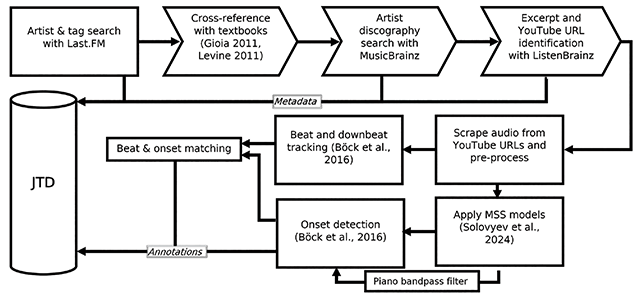
Figure 1
Diagram shows the process for constructing JTD. Arrow block symbols indicate stages where tracks/artists may be removed.
3.1 Performer selection
The criteria used to decide whether an artist should be included in JTD was that they should be both “popular” and “prolific.” With relation to “popularity,” we wanted to ensure that artists would be included only if they were both representative of general jazz listening habits and highly regarded by experts. With relation to “prolificacy,” we wanted to ensure that artists would be included only if they had recorded a significant amount of material in the piano–bass–drums trio format.
3.1.1 Identifying “popular” performers
We searched the Last.fm platform to obtain an overview of jazz listening habits. Last.fm is an online recommendation service that allows users to build profiles of their personal taste by tracking the music they listen to across many streaming platforms. We scraped the names of the top 250,000 performers and groups on Last.fm most frequently tagged by users with the genre “Jazz,” using their official API.1 We ordered by tag count, rather than by plays or favorites, as we wanted to find the most quintessentially “jazz” artists rather than those who fused jazz with other styles.
From the resulting list of performers and groups, we selected only those with the word “Trio” in their name. This left 249 unique performers or groups. While the names of many of the “usual suspects” featured prominently in this list (e.g., Bill Evans, Keith Jarrett), it also included several performers that were mainly known in other genres (e.g., Dee Felice, who accompanied soul singer James Brown when he performed jazz standards) or that mostly composed soundtrack or “stock” music (e.g., Vince Guaraldi, famous for the soundtrack to A Charlie Brown Christmas: see Figure 2).
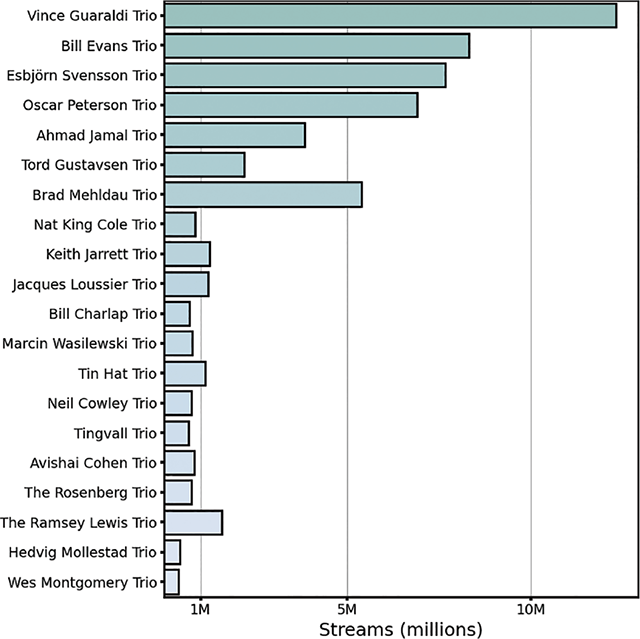
Figure 2
Total streams (“scrobbles”) of all recordings made by the top 20 “trio” artists most frequently tagged as “Jazz” on Last.fm.
We then cross-referenced the Last.fm results against two major jazz textbooks, keeping only those artists that received a mention in the discographies of either Ted Gioia’s The History of Jazz (2011) or Mark Levine’s The Jazz Piano Book (2011). The intention here was to capture artists regarded highly by jazz experts. We note, however, that the retrospective nature of these textbooks could have meant that performers who have become active only in recent years (or, indeed, in the time since their publication) were excluded; future revisions of JTD may use subsequent editions of both textbooks.
This narrowed the total number of groups to 33, all of which were named after a single musician (e.g., the Oscar Peterson Trio). This musician would have led the ensemble and typically composed the majority of the compositions they would play. Two bandleaders were bassists (Dave Holland and Ray Brown) and the remainder were pianists; no bandleaders were drummers.
3.1.2 Identifying “prolific” performers
Next, we turned to searching the MusicBrainz service to acquire a more detailed summary of each bandleader’s recorded discography. MusicBrainz is a community-driven service that provides a comprehensive and open index of discographical metadata (including artist names, recording locations, and release dates) and is commonly used in music information–retrieval tasks. We scraped MusicBrainz using their API to gather metadata relating to every individual recording ever made by each of our 33 bandleaders.2 This resulted in the identification of 18,504 recordings.
We removed recordings that (1) were duplicated across several releases (for instance, those that also appeared on compilation albums), (2) did not contain a complete trio lineup or that included multiple musicians performing on one instrument (for example, a “four hands” piano recording), (3) featured a musician doubling on a second instrument (for instance, a pianist who also played synthesizer or a drummer who played auxiliary percussion), and (4) contained keywords in their title that suggested that they were incomplete performances (e.g., “breakdown,” “outtake,” “false start”).
Four of the 33 bandleaders recorded less than an hour’s worth of material in the trio setting; amongst these, Dave Brubeck, Count Basie, and Joe Zawinul were all better known for their work leading larger ensembles (e.g., quartets, big bands), while Art Tatum worked mainly in a trio of piano, bass, and guitar. After omitting the recordings by these bandleaders, 4,659 tracks remained.
3.2 Recording selection
3.2.1 Inclusion criteria
To obtain a consistent set of tracks that could be analyzed reliably by our automated pipeline, we defined inclusion criteria to compare each recording against before including it in JTD. A track must have had: (1) an approximate tempo between 100 and 300 quarter-note beats-per-minute (BPM), assessed by tapping along to the opening measures of the performance; (2) a clear quarter note pulse, with a time signature of either three or four beats per measure (and with no changes in meter); (3) an identifiable piano solo, accompanied by bass and drums, with no interruptions in the ensemble texture (i.e., “solo breaks”); (4) an uninterrupted “swing eighths” rhythmic feel; and (5) a link to the recording on YouTube.
Additional criteria were specified for each instrument in the trio. During their solo, pianists must have played on acoustic instruments (rather than, e.g., synthesizer or “Rhodes” piano) and without any external FX (e.g., reverb, distortion). Bassists must have played on an unmanipulated acoustic instrument using their fingers or a plectrum, not a bow. Drummers must have used a traditional “traps” kit (snare and kick drums; multiple cymbals, including hi-hat, ride, and crash; tom-toms), without auxiliary percussion (e.g., shakers, maracas). The drums must also have been played using sticks, rather than wire brushes or cloth mallets.
These requirements were included so as to (1) ensure that all notes had clear onset times and (2) maximize the acoustic similarity between the recordings in the dataset and the distribution of (pop, rock) material typically used to train audio source separation models.
3.2.2 Metadata curation
For the recordings that met the inclusion criteria, we combined the metadata scraped from MusicBrainz with additional fields compiled manually, including timestamps for the beginning and the ending of the piano solo, the position of individual instrument sources across the stereo spectrum, and the time signature. YouTube URLs were scraped from the ListenBrainz service using the track identifiers returned from MusicBrainz and manually corrected in the case of any false positives. Audio was downloaded from the URLs, trimmed to the piano solo, and stored in a lossless format with a sample rate of 44.1 kHz.
We elected to include only audio from piano solos, as this is typically the only section in a performance where every musician would be expected to improvise. For instance, in the “head” (melodic statements that occur at the beginning and ending of “straight ahead” jazz performances), the material is pre-composed; whereas in bass or drum solos, the accompanying musicians may choose not to play (Monson, 1996).
Of the 4,659 recordings that were evaluated, 1,294 (27.8%) were included in JTD. The combined duration of all piano solos in these recordings was 44.5 h (Figure 3). These recordings were made between 1947 and 2015, with a median recording year of 1972. The vast majority (93%) had a time signature of four beats per measure.
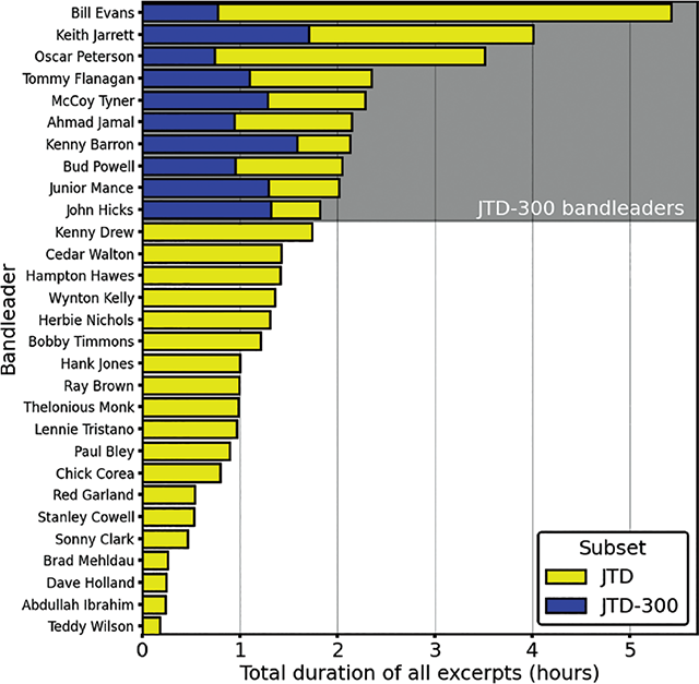
Figure 3
Duration of piano solo excerpts by all bandleaders: bar color indicates subset (either JTD or JTD-300).
The recordings in JTD featured 34 different pianists, 98 bassists, and 106 drummers. Bassist Ray Brown and drummer Ed Thigpen performed together as a rhythm section on the largest number of individual recordings (94). Of those who were not also the leader of their own trio, bassists Ron Carter and Sam Jones accompanied the largest number of different pianists (seven), while drummer Roy Haynes accompanied six pianists. Figure 4 shows the number of tracks by the 10 performers on each instrument with the greatest number of recordings in JTD.
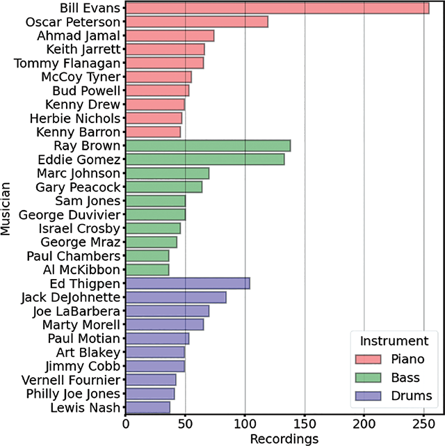
Figure 4
The number of tracks featuring the 10 performers on each instrument with the most recordings in JTD.
JTD-Brushes
Excluding recordings where the drummer used wire brushes resulted in the removal of 973 tracks scraped from MusicBrainz. To address this imbalance, we created a separate set of annotations for tracks that were rejected from JTD only because of the use of brushes. We define this related database as JTD-Brushes. Note that the recordings in JTD-Brushes were not curated to the same extent as those in JTD: the full recording was used, rather than only the piano solo, and the time signature was estimated by the beat tracker automatically, rather than being provided beforehand. The duration of the recordings in JTD-Brushes was 79 h. While the remainder of this article focuses on the curated JTD, we envisage that JTD-Brushes may be of use in developing, for example, beat tracking or “soft” onset detection models that can cope with a broader variety of drumming techniques.
3.3 Class imbalance
A side effect of our inclusion criteria was that bandleaders who worked most frequently in the acoustic “swing” style were overrepresented in the JTD. Conversely, those who worked across a variety of styles or who frequently incorporated electronic elements into their music had very few recordings that met the inclusion criteria. The three bandleaders with the most audio in the JTD were Bill Evans (5.5 h), Keith Jarrett (4 h), and Oscar Peterson (3.5 h). Meanwhile, Abdullah Ibrahim, Brad Mehldau, and Dave Holland were each represented in the JTD by less than half an hour of audio.
This class imbalance could prove problematic were predictive models to be trained on the JTD. To that end, we created a subset of JTD (defined as JTD-300) that includes an equal number of recordings from the 10 bandleaders with the most audio in JTD, sampled chronologically across the duration of their careers. Together, recordings led by these 10 musicians—all of whom were pianists—made up 62.6% of the total duration of audio in JTD (see Figure 3).
For each of these bandleaders, we sorted their tracks in JTD chronologically by the date of recording. In cases where a full date could not be obtained from MusicBrainz, a track was estimated to have been made either midway through the month (in cases where both a month and a year were given) or the year (when only a year was given) it was recorded. In cases where multiple dates were given for one track (i.e., when an album was recorded over a period of time, without dates being assigned to individual tracks), we took the midpoint of these dates. If no dates were provided at all, the track was excluded from selection.
Next, we sorted each track into one of 30 equally spaced bins; the left edge of the first bin coincided with the date of a bandleader’s earliest recording, and the right edge of the final bin with the day of their final (or most recent) recording. Tracks were ordered within each bin by the proximity of their recording date to the midpoint of that bin; if multiple recordings were made on the same day, they were arranged following the order in which they appeared on their original release. We then included the first track from each bin in JTD-300: in cases where a bin was empty, we added an additional track from the first bin, then the second bin, and so on, until 30 tracks were obtained for each bandleader.
The combined duration of the audio in JTD-300 was 11.75 h (26.4% of the duration of JTD). As with JTD, these recordings were made between 1947 and 2015, with a median recording year of 1977.5. The distribution of recording years included in JTD-300 was comparable with JTD (Figure 5). Similar to JTD, 95% of JTD-300 recordings had a time signature of four beats per measure. We envisage that JTD-300 will most likely be of use in performer identification tasks or analyses of chronological trends in improvisation practice. Tasks that do not require balanced class sizes may be better accomplished using the full JTD.
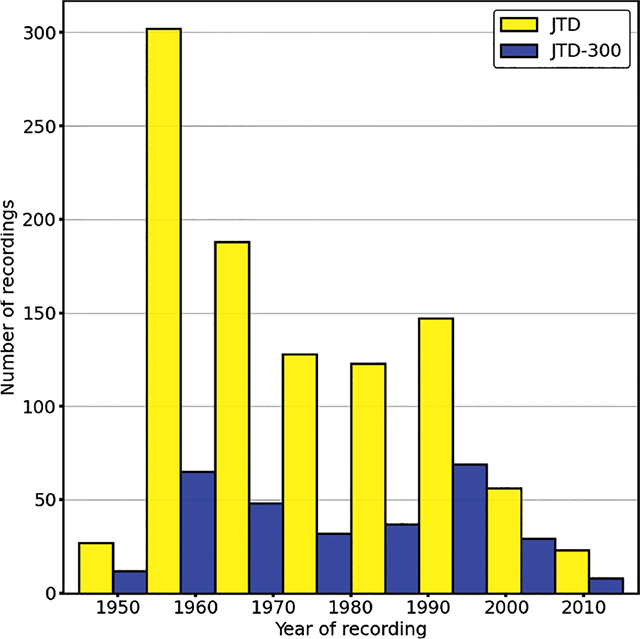
Figure 5
Histogram grouping number of tracks by year of recording: bar color indicates subset.
4. Annotation
4.1 Source separation
4.1.1 Audio channel selection
Before the development of full-spectrum stereophonic panning in the 1970s, audio signals could be panned only to the left or the right speaker output or to both speakers (center channel). For tracks in the JTD where at least one instrument in the trio was hard-panned in this manner (39%), source separation was applied independently to the left and right monaural signals alongside the center output. The required channel was identified manually for each instrument (see 3.2.2).
4.1.2 Model selection
The ZFTurbo audio source separation model (Solovyev et al., 2024) was used to separate each track in the JTD into four sources: “bass,” “drums,” “vocals,” and “other.” This model combines three existing source separation models and achieved the first prize in a recent community sound demixing competition (Fabbro et al., 2024).
4.1.3 Audio filtering
As the ZFTurbo model was not trained explicitly to separate piano audio, we used the “other” source (consisting of the residual audio after removing every other source from the mixed signal) for this instrument. This meant it was possible that audio from the bass and the drums could have “bled” into this track, which would have affected the performance of our downstream annotation pipeline.
To mitigate this possibility, prior to annotation we filtered the “other” source using a second-order Butterworth bandpass filter. Our goal was to attenuate frequency bands that could also be occupied by the drums and the bass while minimizing any damage to the quality of the piano audio. The filter was set to attenuate frequencies outside the range of 55–3520 Hz, equivalent to a six-octave span from A1 to A7: as shown in Edwards et al. (2023), the vast majority of note events in jazz piano performance typically fall within this range.
We demonstrate in 4.3.3 that filtering the piano audio improved the accuracy of our onset annotation pipeline compared to using the raw audio and that this particular frequency range performed better than an alternative, quantitatively “narrower” range.
4.1.4 “Vocal” source
Another possibility was that the unmixed “vocal” source could contain piano audio, which would necessitate summing it with the “other” source. We manually inspected the “vocal” source across a sample of 34 recordings sampled from JTD-300 (see 4.3.1). In all of these cases, the “vocal” source was either silent or contained vocalizations of the musicians (or, occasionally in the case of a live recording, members of the audience) reacting to the performance. Therefore, the “vocal” source was not used for downstream data extraction.
4.2 Data extraction
Our data extraction pipeline consisted of three components: (1) an onset detection algorithm applied to each separated audio source (except “vocal”), (2) a beat and downbeat tracking algorithm applied to the raw audio mixture, and (3) an algorithm to match onsets with their nearest beat in order to assign a metrical interpretation to each onset. Our implementations of (1) and (2) were from the Python madmom package (Böck et al., 2016).
4.2.1 Onset detection
The “CNNOnsetDetector” function in madmom was used to detect onsets in the isolated audio obtained for each instrument in the trio. This algorithm placed first in the most recent MIREX onset detection competition.3 A convolutional neural network (CNN) is fed spectrogram frames of audio (at the default rate of 100 frames per second) to obtain an onset activation function; this envelope is then smoothed using a moving window, and onsets are identified as local maxima higher than a predetermined threshold. Both the window size and the peak-picking thresholds were optimized separately for each instrument class in JTD (see 4.3.2). In 4.3.3 we demonstrate that for detecting onsets in the JTD piano audio, this algorithm outperformed both an existing automatic piano transcription algorithm (Kong et al., 2021) and a naive spectral flux approach.
4.2.2 Beat detection
The “DBNDownBeatTracker” function in madmom was used to detect the position of quarter note beats and downbeats in the audio mixture. This algorithm placed first in the most recent MIREX beat tracking competition.4 A recurrent neural network (RNN) is applied to frames from an audio spectrogram to distinguish among beats, downbeats, and non-beat classes; a dynamic Bayesian network then infers meter from the RNN observations (using the default rate of 100 frames per second). Meter changes cannot be detected by this algorithm, which led us to incorporate into the inclusion criteria that tracks must not have meter changes (see 3.2.1).
We applied this algorithm multiple times to a single track. First, the default parameters specified by the authors were used, with the tempo allowed to vary between 100 and 300 quarter note beats-per-minute (as specified in the inclusion criteria). This resulted in the timestamps changing tempo frequently due to the lack of constraint in the parameter settings. We extracted the duration of successive timestamps and removed outliers according to the 1.5 IQR rule. Finally, we re-ran the beat tracking algorithm using the first and third quartile of the cleaned inter-beat interval array as the new minimum and maximum tempi. The total number of iterations that this process ran for was optimized for the recordings in JTD (see 4.3).
The downbeat classes estimated from the RNN were then combined with the detected beat positions and the time signature for the recording in order to assign measure numbers to every detected timestamp.
4.2.3 Beat-Onset matching
The final stage of our detection pipeline involved matching every beat with the nearest onset detected in each instrumental source. The size of the window used to match any given onset to the nearest beat varied depending on the tempo of a track. Onsets played up to one 32nd note before and one 16th note after any given timestamp were included within the window; whichever onset had the smallest absolute distance to the beat was understood to mark the pulse. If no onsets were contained within a window, then the musician was considered to not have marked the pulse at that timestamp.
4.3 Validation
4.3.1 Ground truth annotations
To evaluate the effectiveness of our annotation pipeline, we manually annotated beat, downbeat, and onset positions across a representative subsample of tracks. In particular, we wanted to check whether the pipeline was resilient across a range of possible recording qualities and also across the different styles of the musicians that are represented most prominently in JTD. Consequently, we adopted a systematic approach, annotating the earliest, middle, and final recordings made by each of the 10 bandleaders in JTD-300. Owing to his overrepresentation in JTD, we also annotated an additional four tracks by Bill Evans (selected randomly from JTD-300)—enough to ensure that the percentage of recordings led by Evans in the subsample (20.6%) was equivalent to JTD (19.6%).
Two of the authors and one research assistant created the reference annotation set. The annotations of the assistant were checked for accuracy by the lead author. The combined duration of the 34 recordings in the subsample was 72 min. The median recording year was 1975, comparable with both JTD and JTD-300 (see 3.2.2, 3.3), and the range of recording years was identical (1947–2015). Similar to JTD and JTD-300, in this annotated subsample 88% of recordings had a time signature of four quarter notes per measure.
4.3.2 Validation results
The performance of the pipeline was determined by considering the proportion of detected annotations that occurred within a 50 ms window of a ground truth annotation. For every track in the subsample, separate precision, recall, and F-measures were computed for each class: (1–3) the onsets within each unmixed instrumental source, (4) the quarter note beats, and (5) the downbeats within the audio mixture. When F = 1, every onset or beat detected by the pipeline could be matched with a ground truth annotation, with no onsets or beats unmatched.
We applied the gradient-free, nonlinear optimization algorithm “subplex” (Rowan, 1990) implemented in the NLopt library to set the parameters of the beat and the onset detection algorithms separately for each audio source.5 In every case, the mean value of F across the entire hand-annotated subsample was treated as the objective function to maximize. Note that for the beat detection algorithm, only the F-measure obtained from evaluating the beat timestamps—not the downbeats—was considered during optimization.
The values of F obtained from the optimized parameter set are shown in Table 2. The performance of the onset detection algorithm was broadly equivalent across instrument classes, with drums performing marginally better than bass and piano. We obtained similar onset detection accuracy to previous work that applied the same algorithm to equivalent multi-tracked datasets (“polyphonic pitched,” mean F = 0.95; “plucked strings,” mean F = 0.90; “solo drums,” mean F = 0.93; see note 3), This indicated to us that the source separation process was unlikely to have caused significant damage (in the form of artifacts, etc.) to the audio, to the point that onset detection algorithms trained on multi-tracked recordings could not also be applied to JTD.
Table 2
Optimized results per instrument, showing F-measure, precision, and recall (mean ± SD).
| Piano | Bass | Drums | Beats | Downbeats | |
|---|---|---|---|---|---|
| F | 0.93 ± 0.03 | 0.93 ± 0.05 | 0.95 ± 0.03 | 0.97 ± 0.05 | 0.63 ± 0.44 |
| P | 0.93 ± 0.04 | 0.94 ± 0.04 | 0.96 ± 0.04 | 0.97 ± 0.05 | 0.63 ± 0.44 |
| R | 0.93 ± 0.04 | 0.93 ± 0.07 | 0.94 ± 0.04 | 0.97 ± 0.05 | 0.63 ± 0.44 |
While the beat tracking results indicated good performance, downbeat tracking was noticeably worse. To understand why, we inspected all tracks where downbeat tracking F = 0.0, while beat tracking F > 0.95 (i.e., the downbeats were out-of-phase). We observed that in the majority of these cases, metrically “strong” beats were being mistaken for other “strong” beats (i.e., beat 2 and beat 4, in 4/4) rather than for “weak” beats, and vice versa. This suggests that our results may still have some value in the analysis of metrical structure, and we also observed that our results were in line with those obtained from applying the same algorithm to other metrically complex forms of music.6 However, future revisions of JTD may leverage the modular design of our codebase to integrate more sophisticated downbeat tracking algorithms as these are developed.
Finally, we looked at the temporal difference between equivalent automatic and ground truth annotations. The pipeline tended to annotate beats and onsets earlier than the human annotators did; the mean difference in beat location time (algorithm – human) was −4.82 ms (SD = 4.58), and for onsets, the mean difference was −4.53 ms (SD = 3.42). There were no substantial differences among onsets detected for different instrument classes (piano: −5.77 ms; bass: −4.29 ms; drums: −4.53 ms). In context, this variation was likely perceptually sub-threshold and should be negligible in most applications.
4.3.3 Alternative methods
Next, we compared several alternative onset detection methods using the piano audio and the corresponding ground truth annotations for evaluation. These methods were: (1) an automatic transcription model (Kong et al., 2021), which generates MIDI (incorporating both pitch and rhythmic information) from audio; (2) a naive audio signal processing approach, whereby onsets were identified as local maxima from a normalized spectral flux envelope (using the implementation described in McFee et al., 2015); (3) the current approach, without the audio filtering described in 4.1.3; and (4) the current approach, with a quantitatively “narrower” bandpass filter (attenuating frequencies outside the range of 110–1760 Hz—i.e., A2–A6).
Note that as (1) generates multiple MIDI events for what would be regarded perceptually as a single onset (i.e., a chord), near-simultaneous MIDI events within a window of 50 ms were grouped together, with the onset of the earliest event taken as the onset of the whole group. The size of this window was optimized following the method described in 4.3.2, as were the individual parameter sets used to pick peaks from the activation functions returned separately from methods (2–4).
The results from this comparison are given in Table 3. For detecting onsets in the JTD piano audio, the current approach outperformed all four alternatives. In particular, we noted that “narrowing” the bandpass filter seemed to affect the precision-recall tradeoff of the CNN predictions: the narrower filter setting (4), for example, resulted in a lower false positive rate than the settings described in 4.1.3 but a higher false negative rate. The current approach, with filter settings between those of methods (3–4), resulted in approximately equal precision and recall. All three CNN-based methods significantly outperformed spectral flux.
Table 3
Results per method, piano only (mean ± SD).
| MIDI transcription (1) | Spectral flux (2) | CNN: no filtering (3) | CNN: narrow filter (4) | |
|---|---|---|---|---|
| F | 0.77 ± 0.13 | 0.84 ± 0.06 | 0.92 ± 0.03 | 0.92 ± 0.03 |
| P | 0.71 ± 0.16 | 0.79 ± 0.10 | 0.90 ± 0.06 | 0.95 ± 0.03 |
| R | 0.86 ± 0.09 | 0.90 ± 0.04 | 0.93 ± 0.03 | 0.89 ± 0.05 |
The results obtained for method (1) were disappointing, especially when compared to those given by the authors. One possibility was that this model may have overfitted to the acoustic properties of the instrument(s) in its training data and was less resilient to the varied recording conditions contained in JTD. More robust approaches that make use of, for example, augmented training data (see Edwards et al., 2024) may be worth exploring.
Regardless, these MIDI annotations are included in JTD, with the caveat that they may be of greater use in downstream tasks that do not require strict timing accuracy (e.g., in analyzing melodic or harmonic content). The total number of MIDI events was 2,174,833 (~2.5 the number of total piano onsets).
5. Analysis
Across JTD, there were 2,206,413 onsets (piano: 866,116; bass: 543,693; drums: 796,604) and 512,272 beat timestamps, 130,547 of which were labeled as downbeats. On average, a solo contained 669 piano onsets, 420 bass onsets, 616 drums onsets, 396 beats, and 101 downbeats; 87.4% of beat timestamps could be matched to a drum onset, and 82.0% could be matched to a bass onset. Only 71.0% of beats could be matched to a piano onset, which emphasizes that keeping time is not the primary aim of jazz soloists.
5.1 Solo duration
On average, the duration of a piano solo in JTD was 2 min and 3 s. Both the shortest and the longest solos were by Bud Powell, with the shortest lasting only 22 s (Powell, 1956) and the longest lasting 7 min, 17 s (Powell, 1962).
There was considerable variation in the duration of solos played by different pianists (Figure 6). In particular, the later a pianist’s first recording in JTD was made (i.e., the later they began their career), the longer they tended to solo for. For the nine (out of 27) pianists in JTD with the longest average solo durations, the median year that their first recording was made was 1967; for the nine pianists with the shortest average solos, the median year was 1956.
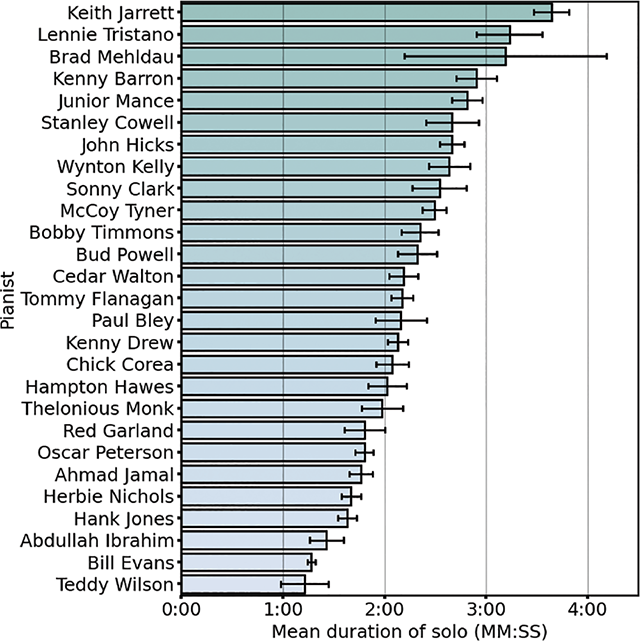
Figure 6
Mean duration of solos by different JTD pianists. Error bars show standard errors.
One possible explanation is that the open-ended formal designs (e.g., modal “vamps,” “time, no changes”) that became popular in jazz during the latter half of the twentieth century proved more suitable for extended improvisation because they did not need to follow the harmonic structure of an underlying “song form” (Gioia, 2011). Changing trends in the music business could provide another explanation: up until the mid-1950s, record companies would often fill albums with multiple shorter recordings rather than longer individual takes so that individual tracks could be released as singles to be played on jukeboxes and radio stations (Priestley, 1991).
5.2 Tempo
Rather than working directly with the timestamps estimated from the beat tracker, we instead defined the location of a “beat” as the mean of all onsets matched to a single timestamp (see 4.2.3). Given our omission of tracks with, for example, a predominant “two-beat” feel (where half notes could conceivably be understood to mark the “beat”) and with “straight” eighths (where these could be felt to mark the beat), these timestamps would be expected to correspond with quarter notes. In cases where fewer than two onsets were matched with a single timestamp (for instance, where at least two instruments played “off” that beat), it was set to missing. At least two instruments played “on” the beat for 88.7% of detected beat timestamps within JTD.
The mean tempo of a recording in JTD was 193.92 BPM (SD = 46.93, Figure 7); this was comparable to the equivalent result calculated using the timestamps estimated from the beat tracking algorithm (mean = 193.70 BPM, SD = 46.59). The slowest performance in JTD had a tempo of 102.10 BPM (Walton, 2010), and the fastest had a tempo of 299.82 BPM (Hicks, 1987).
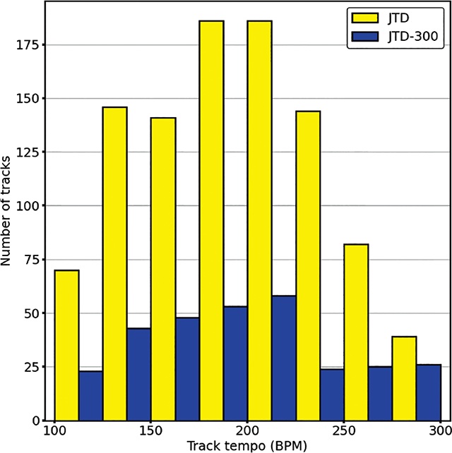
Figure 7
Distribution of tempi (in quarter note beats per-minute).
As measures of tempo stability, for each track we obtained (1) the standard deviation of the tempo normalized by the mean tempo—that is, the percentage fluctuation about the overall tempo (“tempo fluctuation”)—and (2) the slope of a linear regression of instantaneous tempo against beat onset time, with positive values implying acceleration and negative values implying deceleration (“tempo slope”). The average tempo fluctuation was 5.55% (SD = 2.70), whereas the average tempo slope was 0.04 BPM/s (SD = 0.10). This suggests that performances were generally stable, with a slight tendency toward acceleration (with a predicted increase of 1 BPM every 25 s).
There was no correlation between signed tempo slope and unsigned tempo fluctuation: r(1292) = −0.06, p = 0.06; however, there was a positive correlation between unsigned slope (i.e., any global change in tempo, regardless of direction) and fluctuation: r(1292) = 0.37, p < .001. There were also positive correlations between both mean tempo and signed tempo slope, r(1292) = 0.25, p < .001; mean tempo and unsigned slope, r(1292) = 0.60, p < .001; and mean tempo and fluctuation, r(1292) = 0.24, p < .001. This suggests that performances that had a faster pace tended to involve a greater magnitude of tempo change than those that were slower, and that faster performances were also less stable overall.
5.3 Swing
In jazz, “swing” refers to the division of the pulse into alternating long and short intervals. Expressed in Western notation, the long interval is typically written as a quarter note triplet, and the short interval is written as an eighth note triplet. Empirically, swing can be measured by taking the ratio of these long and short durations (the swing or “beat–upbeat ratio,” commonly expressed in binary logarithmic form in the literature). For notated “swung” eighths, the beat–upbeat ratio = 2:1 (log2 = 1.0); for “straight” eighths (i.e., the equal–equal subdivision of the beat), the beat–upbeat ratio = 1:1 (log2 = 0.0).
We searched our database for all discrete groupings of three onsets where the first and the last had marked the quarter note pulse. The total number of such groupings was 417,278. Following Corcoran and Frieler’s analysis of the WJD (2021), we classified ratios above 4:1 (log2 = 2) and below 1:4 (log2 = −2) as outliers, which resulted in the exclusion of 2.10% of these groupings. The final number of beat–upbeat ratios in the dataset was 408,506 (piano: 151,640; bass: 47,115; drums: 209,751).
5.3.1 Differences in swing between instruments
To evaluate the differences in swing ratio among the instruments in the trio, we smoothed the distribution of beat–upbeat ratios obtained for each instrument through kernel density estimation (calculating the bandwidth using Silverman’s rule-of-thumb). We then applied the peak-picking algorithm from the SciPy library, using the default parameters, to obtain the local maxima of the smoothed curve.7 Confidence intervals for these peaks were generated by bootstrapping over the results from different bandleaders (n = 10,000 replicates).
For the piano, we found one peak in the density estimate, corresponding to a log2 beat–upbeat ratio of 0.37 (beat–upbeat ratio: 1.44:1, 95% CI: [0.15, 0.43]). For the bass, we found two peaks, corresponding with log2 beat–upbeat ratios of 0.06 (1.06:1, [0.03, 0.13]) and 1.23 (3.41:1, [1.15, 1.27]). For the drums, we also found two peaks, at log2 beat–upbeat ratio −0.91 (0.40:1, [−1.15, −0.70]) and 1.18 (3.25:1, [1.13, 1.23]). These density estimates and the corresponding peaks are shown in Figure 8.
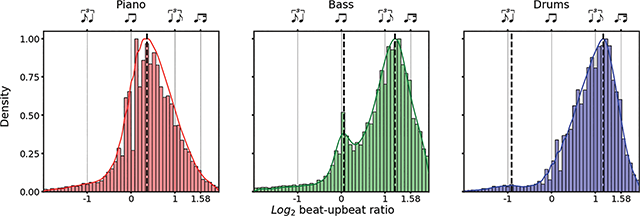
Figure 8
Each panel shows the distribution of log2 beat–upbeat ratios among instruments across JTD, normalized such that the height of the largest bar in each panel is 1. Dotted vertical lines show peaks of the density estimates; straight lines correspond to the musical notation given along the top of the panel.
This analysis suggested that (1) all instrument classes primarily targeted long-short divisions of the beat, with the percentage of total log2 ratios > 0.0 = 88.6% (piano: 81.9%; bass: 89.1%; drums: 93.4%); (2) pianist beat–upbeat ratios were closer to notated “straight” than “swung” eighths, judging by the peak of their density estimate; (3) in contrast, the larger of the two peaks in the bass and the drums density estimates suggested that both instruments tended toward higher beat–upbeat ratios than would be implied by notated swing eighths alone.
The fact that soloists tended to swing less than the expected 2:1 ratio—while accompanists swung “more” than this—has been well documented. Butterfield (2010) has, for instance, suggested that relatively “straight” eighth notes help to maintain forward momentum in a soloist’s improvisation, whereas the more “swung” eighth notes of the accompaniment helps to facilitate hierarchical beat perception. We include examples of piano playing with successive beat-upbeat ratio values below 0.0 in the supplemental materials.
We also noted that the mean beat–upbeat ratio for piano soloists in JTD (1.53:1) was close to that obtained for “SWING” tracks in WJD (1.41:1; see Corcoran and Frieler, 2021). Caution should be taken when interpreting these results, however, as WJD contains a greater variety of tempi and solo instruments than JTD.
5.3.2 Effect of tempo on swing
Next, we considered the relationship between swing and the tempo of a performance. We fitted a linear mixed effects model, predicting a performer’s mean log2 beat–upbeat ratio using the mean tempo of the recording (standardized through z-transformation), their instrument, and the interaction between tempo and instrument as fixed effects (piano = reference category). Bandleader was used as a random effect (slopes and intercepts). An individual musician’s performance was excluded if 15 ratios could not be obtained, resulting in the exclusion of 471 individual performances out of 3,865 (piano: 30; bass: 401; drums: 40).
An increase in mean tempo was a significant predictor of a decrease in mean beat–upbeat ratio for a recording (Figure 9), with a 1-SD change in BPM associated with a decrease of −0.14 mean log2 beat–upbeat ratio (p < .001, 95% CI: [−0.16, −0.12]). This suggested that it became harder for musicians to articulate long–short subdivisions of the quarter note as its duration decreased. This “straightening” effect has also been observed in analyses of both WJD (Corcoran and Frieler, 2021) and Filosax (Foster and Dixon, 2021).
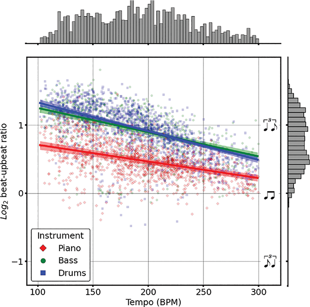
Figure 9
Markers show mean log2 beat–upbeat ratio and tempo; solid lines show predictions (without random effects); and shaded areas show 95% confidence intervals (obtained via bootstrapping over data from different pianists, N = 10,000)
There were significant negative interactions between instrument and tempo for both the bassist ( = −0.06, p < .001, 95% CI: [−0.09, −0.04]) and the drummer ( = −0.10, p < .001, 95% CI: [−0.12, −0.08]). Put differently, the “straightening” effect was more severe for accompanying, rather than soloist, roles. The amount of variance in the data explained by both the fixed and the random effects of the model was 61.9%, compared to 58.8% for the fixed effects only. This suggested only minimal differences in the effect of tempo on swing among ensembles.
5.3.3 Effect of recording year on swing
We fitted the model described in 5.3.2 with an additional fixed effect of recording year (standardized via z-transformation) and the interaction between year and tempo. Increases in recording year had no significant main effect on mean log2 beat–upbeat ratio ( = 0.01, p = 0.44, 95% CI: [−0.02, 0.05]), and there was no significant interaction between year and tempo ( < 0.01, p = 0.79, 95% CI: [−0.01, 0.01]). Including the year of recording in the model also resulted in minimal change to the amount of variance it explained (conditional R2 = 62.8%; marginal R2 = 59.3%).
This suggested that the year a track was recorded had minimal impact on the levels of swing displayed by the musicians. These results should not be taken as indicative of global trends in swing timing, however, as the recordings in JTD are (by design) mostly representative of the “straight ahead” jazz style practiced throughout the last century. Prior analysis of the WJD has demonstrated tangible differences in swing among different styles of jazz (Corcoran and Frieler, 2021).
5.4 Synchronization
Synchrony can be defined as the difference among onsets that demarcate the same musical event (e.g., a quarter note beat). While it can be expressed in “raw” units (milliseconds, frames), we expressed synchrony as a percentage of the duration of a single quarter note at the tempo of a track, which allows for comparison across performances made at different tempi. For example, a value of +25% would imply that one musician played a 16th note later than another musician did.
In Figure 10, we show kernel density estimates for the relative position of beats by each instrument on a circle: the flow of time unfolds in a clockwise direction, with values shifted such that the mean position of the drummers’ first beat aligns with 0 degrees.
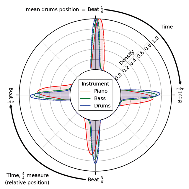
Figure 10
Diagram shows kernel density estimates for the relative position of beats by each instrument, indicated by color. Density estimates are scaled such that the maximum height of the curve for each instrument is 1.
We calculated the synchrony between all pairs of instruments in the trio at every quarter note, across all tracks in JTD. Confidence intervals were again obtained by bootstrapping over the results obtained for different bandleaders (n = 10,000). Bassists played 1.5% (95% CI: [1.0, 2.0]) of a quarter note later than drummers, on average. This close synchronization between bass and drums helps anchor the jazz soloist’s performance (Butterfield, 2010). On average, pianists played 5.6% (95% CI: [4.8, 6.3]) of a quarter note later than drummers and 4.0% ([3.2, 4.9]) later than bassists, approximately a 64th note (6.3%) delay.
This delay of the soloist relative to the accompaniment has been observed frequently in the literature on jazz improvisation (e.g., Butterfield, 2010). To investigate whether it depended on the tempo of a performance, we fitted a mixed effects model that predicted the mean asynchrony between pianist and accompaniment using as fixed effects the tempo (z-transformed), the accompanying instrument (bass or drums), and the interaction between tempo and accompanying instrument (bass = reference category). Bandleader was used as a random effect (slopes and intercepts).
Increased tempo predicted significantly reduced asynchrony; for every SD increase in tempo, mean pianist-accompaniment asynchrony decreased by −0.4% of the duration of a quarter note beat (p < .05, 95% CI: [−0.7, −0.1]). There was a significant interaction between accompanying instrument and tempo ( = 0.3, p < .01, 95% CI: [0.1, 0.5]). Faster performances thereby had tighter soloist-accompaniment synchronization than did slower ones, with this effect being stronger for piano–bass synchronization than for piano–drums.8
The size of this effect was relatively small, however, with less than a 256th note difference (1.56% of a quarter note beat) in predicted mean asynchrony between pianist and bassist at both the slowest and fastest tempo in the corpus. The amount of variation in the data explained by the fixed effects was only 5.6%, compared with 29.3% for fixed and random effects—suggesting that differences among ensembles could be a more substantial source of variation.
6. Conclusion
We presented JTD, a new dataset of 44.5 h of jazz piano trio recordings with automatically generated annotations. Appropriate recordings were identified by scraping user-based listening and discographic data; a source separation model was applied to isolate audio for piano, bass, and drums; annotations were generated by applying various automatic transcription, onset detection, and beat tracking algorithms to the separated audio. Onsets detected by the pipeline achieved a mean F-measure of 0.94 when compared with ground truth annotations.
We encourage the use of JTD in tasks including performer identification, expressive performance modeling, structure analysis (using the piano solo timestamps), and as a benchmark to compare automatic transcription algorithms. JTD-Brushes may also prove useful in developing, for example, beat tracking models that can cope with a broader variety of drumming styles and “soft” onsets. Comparison between accompanied and unaccompanied jazz piano playing may be another fruitful direction for research. The lower accuracy of the automated downbeat annotations compared to both onsets and beats could also inspire the development of downbeat trackers better suited for the jazz genre.
We can foresee some limitations of our work. Our inclusion criteria were particularly strict, which necessitated identifying tracks manually. Automated tagging methods (e.g., distinguishing between a drummer’s use of brushes or sticks) could enable more efficient data collection. JTD also shows an imbalance toward male performers; exceptional inclusions could be made in future revisions to include prolific female musicians who did not appear in the Last.fm search results or jazz textbooks. Finally, we do not include MIDI transcriptions of the bass and drums as we do for the piano, but this omission offers an exciting opportunity for future work, as models capable of performing these tasks continue to develop in sophistication.
Many of the recordings contained in JTD are under copyright and cannot be released publicly; however, we have made the annotations available for download and provide source code to align these with the recordings.9 The design of this code is modular, enabling JTD to be updated easily as the state-of-the-art in the various tasks involved in the annotation pipeline improves. We have also developed a web app including a variety of interactive resources that enable JTD to be explored without having to download it.10
Notes
[9] It is also important to be aware of how, at faster tempo values, the slight variation in onset detection accuracy among instrument classes could also have had an impact on these results. At the mean tempo in JTD, the 1.5 ms difference between bass and piano annotation was equivalent to 0.5% of the duration of a quarter note.
Acknowledgements
The authors express their thanks to Tessa Pastor and Reuben Bance for their help in constructing the dataset.
Competing Interests
The authors have no competing interests to declare.
Author Contributions
HC: conceptualization, methodology, software, validation, formal analysis, investigation, data curation, visualization, writing – original draft, writing – review & editing
JLS: conceptualization, methodology, investigation, writing – review & editing
IC: conceptualization, writing – review & editing, supervision
PMCH: conceptualization, writing – review & editing, supervision
Additional File
The additional file for this article can be found as follows: