
1. Introduction
Many tasks in the field of music information retrieval (MIR), like automatic music transcription or fundamental frequency (F0) analysis, become significantly easier when separated, monophonic audio signals of individual instruments and voices are available. Similarly, music post-production and mixing rely on multi-track recordings to selectively apply audio effects and balance levels. The singing voice is often particularly challenging in those scenarios, due to its large dynamic range and possibility for nuanced expression. While in popular music the separation into monophonic multi-track signals can often be accounted for in the recording process, e.g., by consecutively recording individual singers with a close-up microphone (CM), this is not always possible or desirable. In order to facilitate the natural interaction (in terms of timing, expression, intonation, etc.) between musicians, voices, and/or room acoustics, it may instead be preferable or even necessary to record multiple musicians or instruments at the same time and in the same space. This way, a choir performing in a church, an ethnomusicological field recording of a vocal ensemble, or a singer-songwriter accompanying themselves on a guitar can become challenging for computational analysis and post-production.
Larynx microphones (LMs) provide a practical way to obtain almost crosstalk-free signals of the voice by picking up vibrations at the throat. By design, such a sensor is insensitive to sound waves transmitted through the air and therefore to other interfering sound sources in the environment. However, the LM signal quality is typically degraded by a limited frequency response as well as missing effects of the vocal tract, i.e., the contribution of the oral and nasal cavity responsible for vowel and consonant formation, which are only indirectly picked up at the throat. This limits applications of LMs to cases where audio quality is not a primary concern, like radio communication in noisy environments.
In this paper, we explore the task of singing voice reconstruction (SVR), which aims at obtaining high-quality recordings of singing voice using impaired signals as the input. By using the new term SVR, we want to emphasize important differences to related and established tasks in the research fields of signal processing and MIR, like speech enhancement or singing voice synthesis. In particular, the focus on the singing voice requires careful treatment and preservation of expressive parameters, while at the same time such recordings often include many highly correlated interfering sources. With a focus on SVR from larynx microphone signals (referred to as LM-SVR in the following), we consider a particular SVR scenario in this paper: reconstructing a high-quality singing voice recording — as it could be recorded with a typical CM in ideal conditions — from a monophonic LM signal, thus circumventing the problem of crosstalk during recording, while faithfully retaining the nuanced vocal expression captured in the original signal. Such a reconstructed recording could then be used for downstream applications like mixing or analyzing it with computational systems that require high-quality input, as outlined in Figure 1.
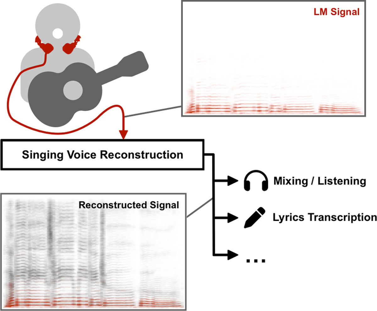
Figure 1
Conceptual overview of SVR from LM signals. Time-frequency representations of an exemplary LM signal and the corresponding reconstructed signal are depicted in red and grey, respectively.
Beyond introducing this novel MIR task, we make three main contributions in this paper. First, we introduce the Larynx Microphone Singer-Songwriter Dataset (LM-SSD), a collection of twelve pop songs performed by four amateur singers accompanied by an acoustic guitar, comprising over 4 hours of unique recordings of LM and corresponding CM signals. This dataset may facilitate research on LM-SVR, but also other tasks like source separation or singing voice analysis. Second, we describe a baseline LM-SVR system which is inspired by source-filter models of the vocal tract, using the LM signal as a source signal and learning the control parameters of a time-variant filter with a neural network. Third, we evaluate the baseline LM-SVR system with a listening test and show that this approach improves the subjective quality of the LM recordings, while also improving objective performance in the exemplary downstream task of lyrics transcription.
The remainder of this article is structured as follows. In Section 2, we consider SVR in the context of related signal processing and MIR tasks, Section 3 describes related work and use cases for LMs, and Section 4 introduces LM-SSD including details of the two LM models used that we compare in terms of their signal characteristics and handling. Section 5 describes our baseline system for LM-SVR, complemented by our experiments with a listening test and objective evaluation on a lyrics transcription task in Section 6.
2. Singing Voice Reconstruction
We define singing voice reconstruction (SVR) as the task of obtaining a natural sounding, artifact-free, and broadband signal without crosstalk from an impaired recording of the singing voice, without changing the original expression in the recording. Typical impairments include adverse recording conditions or limitations of the sensor. With that, SVR is related to several established research areas in signal processing and MIR.
Speech enhancement (SE) focuses on the suppression of artifacts, noise, and other interfering sources from an otherwise high-quality speech signal (Vincent et al. 2018). While classical SE methods often rely on additional (e.g., spatial, see Benesty et al. 2008) information about the recorded signals, state-of-the-art SE systems use data-driven approaches to encode the impaired signal in a typically lower-dimensional latent representation and then decode a new, clean speech signal from that (e.g., Serrà et al. 2022). Similar methods have been employed for singing voice synthesis (SVS), where an interpretable latent representation may enable general-purpose synthesis models (Choi et al., 2021, 2022). Naturally, such systems depend critically on the expressivity of the latent representation and the distribution of training examples, as the decoder may not learn to generate a signal with characteristics that are not observable in the training set. This lack of control is particularly problematic for singing voice signals (Cho et al., 2021), as important expressive parameters like F0 are highly variable within individual notes (Dai and Dixon, 2019) and may not be accurately reproduced by SE or SVS systems, even when F0 is explicitly given in the latent representation (Choi et al., 2022).
Furthermore, in music, desired and interfering sources may be highly correlated, for example when multiple musicians are singing in unison. This problem is subject of the MIR task of musical source separation (MSS, Cano et al. 2019). State-of-the-art systems often introduce characteristic artifacts and reach signal-to-distortion ratios of around 8 dB for vocals on popular music recordings (Mitsufuji et al., 2022), so that separately recording individual instruments and voices is still preferable for many use cases. This recording-time separation can be achieved, for example, with LMs. Since these produce band-limited sensor signals, LM-SVR is also related to blind bandwidth extension (BBWE). BBWE aims for the reconstruction of high-frequency content from a clean but band-limited audio signal without additional side information. Systems often focus on a specific signal domain like speech, where successful approaches model aspects of speech production (Schmidt and Edler, 2021). Apart from subjective quality, BBWE can also improve performance of downstream tasks like speech recognition (Li et al., 2019). Adapting such an approach to the singing voice and larynx microphones is one objective of SVR as introduced in this paper.
3. Larynx Microphones
Larynx microphones (LMs), also called throat microphones, are a type of contact microphone. In general, contact microphones are designed to record vibrations of the surface they are attached to, while being insensitive to sound waves transmitted through air. For LMs, this is typically achieved using a piezo-electric sensor placed on the skin of the neck. This way, one can obtain well-separated signals of individual speakers or singers in all kinds of acoustic conditions. The quality of the recorded signal depends on two factors: the properties of the sensor itself and the way that vibrations are propagated from the source through tissue and/or bones to the receiver. Notably, while the vocal fold vibrations are predominant at the neck, some influences of the vocal tract producing formants and consonants are also present as vibrations in neck tissue (Otani et al., 2006), so that for example speech recorded with an LM can become intelligible. A detailed account of the signal characteristics of two particular LM models used for our dataset is given in Section 4.1.3. To get a subjective impression of the signal qualities, we also refer to the online examples accompanying this paper.1
Another sensor type for LMs has been subject of research on non-audible murmur (NAM, Nakajima et al. 2003). Here, the goal is to pick up whispered speech, which is achieved with a condenser microphone embedded in a soft material that is attached to the skin (Shimizu et al., 2009). Similarly, bone conduction microphones are contact microphones that are adapted to the specific impedance of the skull (Henry and Letowski, 2007). While they may provide more flexibility in their positioning (McBride et al., 2011), the quality of the recorded signal for both NAM and bone conduction microphones is generally comparable to that of LMs.
A different technique for picking up the vocal fold vibrations is electroglottography (Herbst, 2020), where the impedance change between open and closed states of the vocal folds is measured. Recordings with this method are particularly insensitive to any influences of the vocal tract and do not contain enough information to reconstruct a speech or singing signal, but can for example be used to measure F0 (Askenfelt et al., 1980).
LMs have shown their utility in a number of applications in speech and music processing. Graciarena et al. (2003) showed that the information from LMs can improve speech recognition in noisy environments. Askenfelt et al. (1980) used LM signals for F0 estimation, which recently received renewed attention in the context of pitch and intonation analysis of Western choir recordings (Rosenzweig et al., 2020). Scherbaum (2016) showed how LM recordings can aid musicological research, e.g. to computationally determine the tonal organization of traditional Georgian music (Scherbaum et al., 2022; Rosenzweig et al., 2022).
4. LM Singer-Songwriter Dataset
As a main contribution of this paper, we introduce the Larynx Microphone Singer-Songwriter Dataset (LM-SSD) and make it publicly available. LM-SSD is a collection of twelve pop songs that we recorded with four different amateur singers accompanied by a guitar, featuring a solo singer for nine songs and a duet for three songs. In total, the dataset consists of 72 takes with a total playback duration of 250 minutes, as detailed in Table 1 below. While similar datasets exist for speech (e.g., Dekens et al. 2008; Stupakov et al. 2009), this is, to our knowledge, the first dataset with singing voice recordings using LMs and a synchronous, high-quality, and crosstalk-free CM signal.
Table 1
Overview of the songs and takes in LM-SSD. C1 and C0 represent the number of takes with and without crosstalk, respectively. Songs marked with * have German lyrics.
| ID | SONG NAME | ORIGINAL ARTIST | SINGER ID | TAKES C1 | LM-A C0 | TAKES C1 | LM-B C0 | DURATION (MM:SS) |
|---|---|---|---|---|---|---|---|---|
| AA | All Alone | Michael Fast | 1M | 1 | 2 | 1 | 2 | 27:03 |
| TS | The Scientist | Coldplay | 1M | 1 | 2 | 1 | 2 | 21:37 |
| YF | Your Fires | All The Luck In The World | 1M | 1 | 2 | 1 | 2 | 24:21 |
| DL | Dezemberluft* | Heisskalt | 2M | 1 | 2 | 1 | 2 | 14:47 |
| BB | Books From Boxes | Maxïmo Park | 2M | 1 | 2 | 1 | 2 | 17:39 |
| NB | Narben* | Alligatoah | 2M | 1 | 2 | 1 | 2 | 11:47 |
| SG | Supergirl | Reamonn | 3F, 1M | 1 | 2 | 1 | 2 | 26:34 |
| OC | One Call Away | Charlie Puth | 3F, 1M | 1 | 2 | 1 | 2 | 19:32 |
| PL | Past Life | Trevor Daniel & Selena Gomez | 3F, 1M | 1 | 2 | 1 | 2 | 17:45 |
| CC | Chasing Cars | Snow Patrol | 4F | 1 | 2 | 1 | 2 | 28:10 |
| BT | Breakfast At Tiffany’s | Deep Blue Something | 4F | 1 | 2 | 1 | 2 | 22:16 |
| LL | Little Lion Man | Mumford & Sons | 4F | 1 | 2 | 1 | 2 | 19:06 |
| Total | 12 | 24 | 12 | 24 | 250:37 |
LM-SSD is designed to provide signals with consistent recording quality and conditions, as well as instrumentation, while variables like sensor choice, singer, song, and crosstalk are varied systematically. Beyond research on LM-SVR and related tasks, the dataset can for example be used for experiments on analyzing LM signals directly (e.g., for F0 estimation), or the evaluation of domain adaptation in data-driven systems (see e.g. Section 6.2). Additional mix tracks for each song, as well as annotated lyrics furthermore enable use cases like experiments with source separation (possibly informed by LM signals) or lyrics transcription. In the following, we will describe the sensors used (Section 4.1), the recording process (Section 4.2) and the content of the dataset (Section 4.3) in detail.
4.1 LM Models Used
In order to analyze differences between sensors, their handling, and their utility for singing voice recordings, we used two LM models for recording the dataset: the commercially available Albrecht AE-38-S2a (LM-A) and a self-made microphone based on TE Connectivity CM-01B piezo-electric vibration sensors (LM-B). A direct comparison of their properties can be found in Section 4.1.3.
4.1.1 LM-A: Albrecht AE-38-S2a
LM-A is a commercially available device built for radio communication in the security sector. It has two contact microphones at either end of a size-adjustable neck brace (see Figure 2, bottom left). With the adjustable brace it suits a variety of neck sizes, even though it tends to have a looser fit on smaller necks, resulting in a higher probability of movement-induced noise. For all recordings, we aimed to position the sensors as close to the larynx as possible while allowing the musicians to be comfortable while singing. The two analog sensor signals are electrically summed by a connection in series, but the manufacturer provides no details on frequency range or other properties of the sensor. We adapt the 3.5mm TRS connector of the device to XLR using a Røde VXLR+, which also converts 48V phantom power to the required supply voltage of 3.8V.
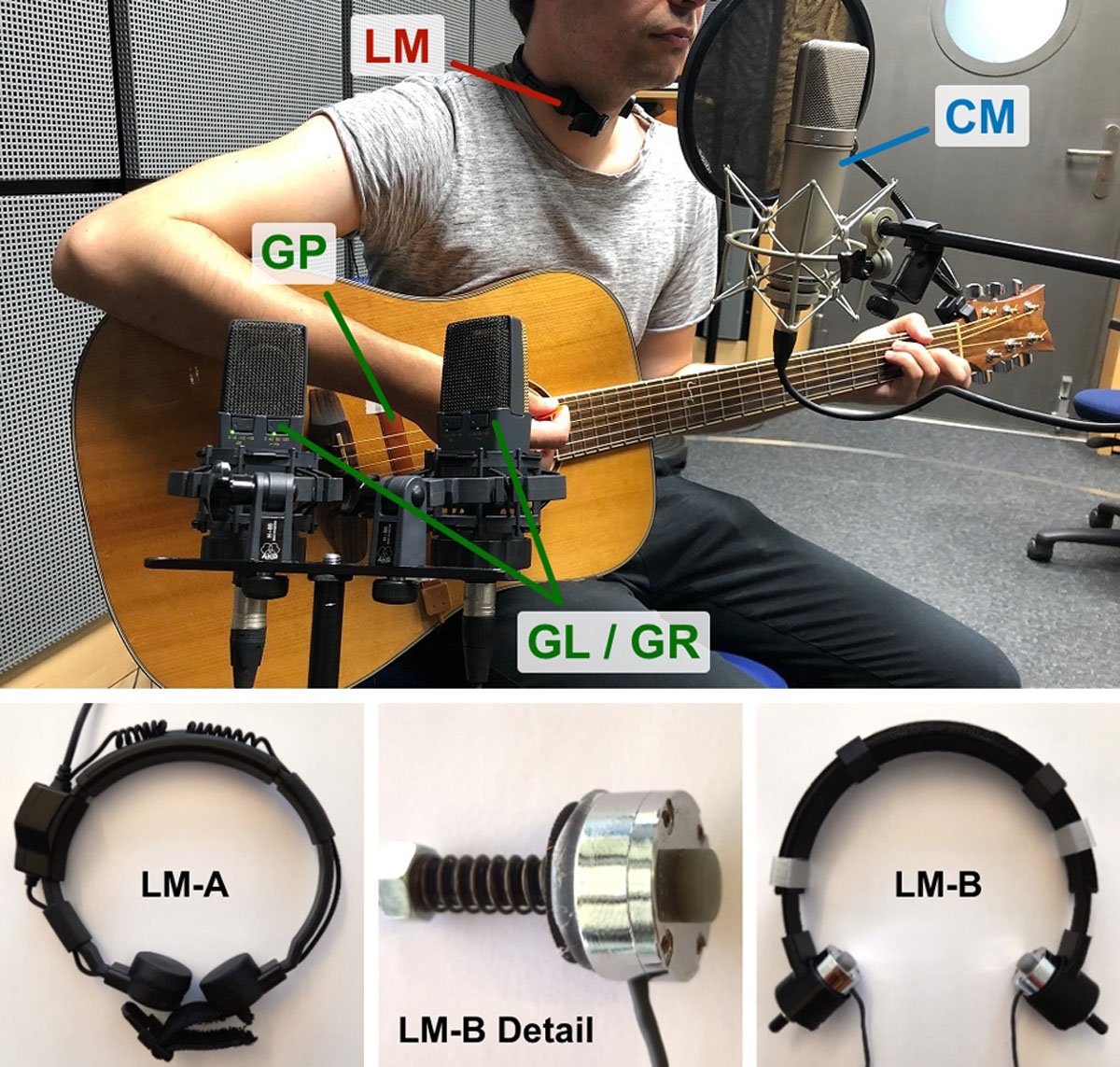
Figure 2
Photograph of the recording setup (top) and detailed depiction of the LMs used (bottom). LM-A: Albrecht AE-38-S2a larynx microphone; LM-B: self-made larynx microphone with TE Connectivity CM-01B sensor; CM: close-up microphone (Neumann U87); GP: guitar pickup (AMG Electronics C-Ducer); GL/GR: guitar stereo left/right (AKG C414).
4.1.2 LM-B: CM-01B
LM-B is a self-made larynx microphone using two piezo-electric vibration sensors (TE Connectivity CM-01B) and a 3D-printed neck brace. The sensor is optimized for detecting body sounds, whose vibrations are transmitted via a small rubber pad on the device. It is marketed with a frequency range of 8 to 2200 Hz (∓3 dB). To achieve comparability with LM-A, we use two sensors on either end of the brace and digitally sum the signals after recording. The sensors are attached to the neck brace with a screw that is glued onto the backside of the sensor and a spring that pushes the sensor lightly towards the skin of the neck (see Figure 2, bottom middle). The sensor contact point can be adjusted and is further away from the larynx than with LM-A, which singers reported to be more comfortable. The neck brace is not adjustable to different neck sizes, but it can be printed in different dimensions, which also makes it possible to specifically fit the brace for individual persons.
4.1.3 Signal characterization & comparison
Obtaining objective measurements of the LM voice signal characteristics is challenging, as the properties of the transmitting medium and the vibration source(s), as well as possible losses at the contact point have to be taken into account. A direct transfer function between source and receiver cannot be measured, because the ground truth “source signal” is not available. Instead, we consider the relative transfer function (RTF) between CM and LM as a first indication of the similarity between the LM signals and traditional microphone recordings. Using an unbiased estimator (see Appendix A.1 for details), we calculate RTF estimates for the two LM models using the crosstalk-free recordings (cf. Section 4.2) from LM-SSD. Results for signals from individual singers (in grey) and their average (in black) are presented in Figure 3, where an RTF value around 0 dB signifies that CM and LM signals tend to have similar energy at a given frequency. The RTF for LM-A remains around 0 dB below 700 Hz and drops off at higher frequencies by –9 dB per octave on average. LM-B boosts low frequencies by up to +20 dB below 20 Hz and the RTF continuously drops towards high frequencies by around –6 dB per octave. Between 80 to 700 Hz, the approximate range of the F0 of male singing voices, energy levels of LM-A and LM-B are fairly similar to the CM signal. The estimates for different singers are similar within ± 5 dB in the relevant frequency range, which is an indication that both LM models are fairly robust w.r.t. fit and exact positioning.
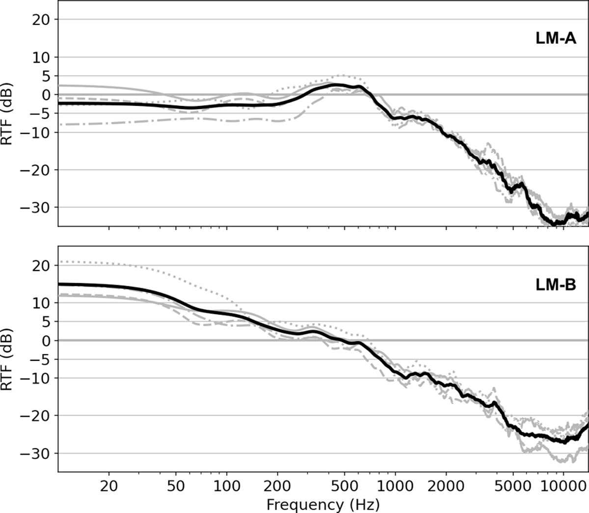
Figure 3
Relative transfer function (RTF) estimates w.r.t. CM for LM-A (top) and LM-B (bottom). RTF estimates for individual singers are shown in grey (1M: solid, 2M: dashed, 3F: dotted, 4F: dash-dotted). The black line indicates the mean RTF across singers for each LM model.
The RTF does, however, not allow conclusions about noise levels and distortion of the LM relative to the CM signal. For that, we can additionally measure the coherence between the two signals, showing whether they are linearly related at a given frequency. When the maximum coherence of 1 is achieved, a linear filter exists to calculate the corresponding CM signal from an LM recording and vice versa. Conversely, minimum coherence of 0 is reached when no linear relationship exists, e.g., when one or both signals are uncorrelated noise or one signal contains non-linear distortions. Figure 4 shows coherence estimates (see Appendix A.2 for details of the method) for the signals from individual singers (in grey) and their average (in black). Between 80 Hz and 3.5 kHz (the range of F0 and the first few harmonics of the recorded voices), the CM and LM signals are somewhat linearly related, but the coherence rarely exceeds 0.6, hinting at the presence of noise and distortion in the LM recordings. The low coherence at low frequencies is due to the singing voice not being present on the CM below F0, while the LMs, particularly LM-B, might still record relevant signal. The mean coherence for LM-B is slightly larger towards high frequencies, which can at least partially be attributed to a stronger distortion in the LM-A signal when singing with higher intensity.2
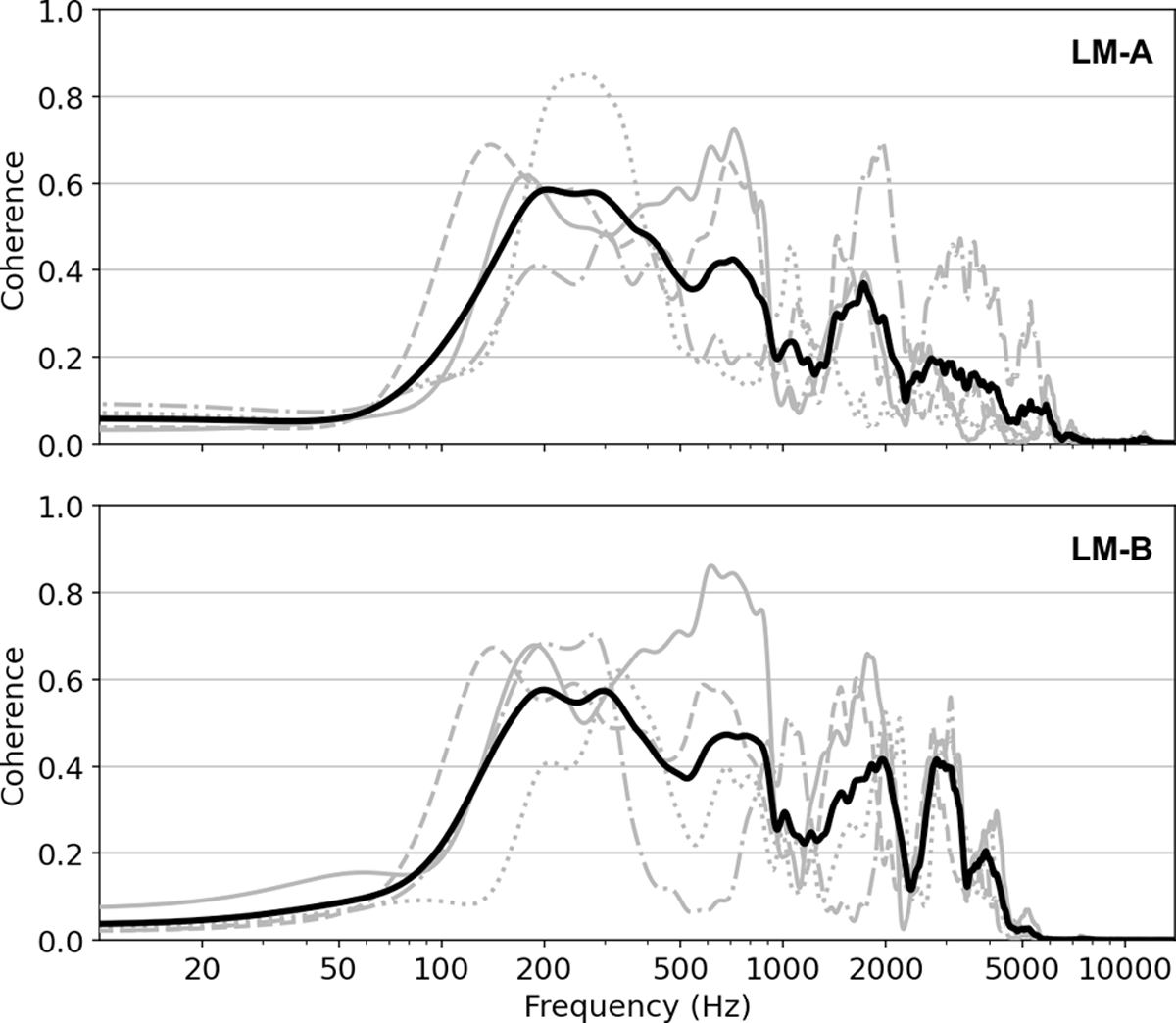
Figure 4
Coherence estimates w.r.t. CM for LM-A (top) and LM-B (bottom). Coherence estimates for individual singers are shown in grey (1M: solid, 2M: dashed, 3F: dotted, 4F: dash-dotted). The black line indicates the mean coherence across singers for each LM model.
Finally, we also measure the sensitivity of each LM w.r.t. interfering sound transmitted through the air. We consecutively record the LM signals while an external noise source is playing and while the wearer is singing, both reaching the same sound level at a fixed measurement position in the room. The level difference between these two recordings gives a relative measure for the “crosstalk sensitivity”, indicating the dampening of surrounding sounds compared to the voice of the wearer. We estimate –60 dB for LM-A and –55 dB for LM-B.
While the objective properties are similar for both LM models, the high-frequency distortion of LM-A at higher volumes also subjectively reduces the signal quality. Furthermore, singers reported higher comfort wearing LM-B, as the contact point of the sensors is less close to the throat, while the self-made construction offers higher flexibility due to the possibility of customizing the neck brace and individually recording left and right sensor signals. On the other hand, LM-A requires only one recorder channel and is more robust in handling (as it is constructed as a single piece without removable parts) and fit (due to the adjustable brace), which can be an advantage, e.g., for field recordings.
4.2 Recording Setup & Procedure
LM-SSD comprises recordings of two male (denoted 1M and 2M) and two female (3F and 4F) university students. All musicians are amateur singers without formal music training and only limited stage or recording experience and consented in writing to the processing and publication of the recordings. Each singer selected three pop songs they felt comfortable with in terms of vocal range and techniques. While 1M and 2M accompanied themselves on the guitar, 3F and 4F were accompanied by a second musicians, while 3F also sang in duet with 1M. Two of the songs have lyrics in German language, while the others are in English. An overview of the songs in the dataset is given in Table 1.
The musicians were recorded in a studio room with little reverberation and optimized acoustics for pop music recording. As depicted in Figure 2 (top), the recording comprises a traditional microphone setup, including a close-up vocal microphone (CM; Neumann U87, set to cardioid) with a pop filter, a stereo close-up microphone pair for the guitar (GL and GR for left and right channel, respectively; AKG C414, set to cardioid) and a guitar pickup microphone (GP; AMG Electronics C-Ducer). In addition, all singers were wearing one of the two LM models (see Section 4.1) at a time to record their voice. Preliminary experiments showed that the optimal positioning of the LM on the neck would be compromised if both LMs were worn at the same time, as both record the cleanest signals when positioned high on the neck and as close as possible to the larynx without becoming uncomfortable for the singer. Note that, depending on the singer’s distance to the CM, there is a small time-varying delay between the CM and LM signals,3 which we do not compensate for in the dataset.
In total, six takes were recorded for each song, three with LM-A (T1–T3) and three with LM-B (T4-T6). Of those takes, the first of each group (T1 and T4) was played with live guitar accompaniment, i.e. the guitar playing in the same room as the singer (singers 1M and 2M accompanied themselves, whereas 3F and 4F were accompanied by a second musician). In takes T2, T3, T5, and T6, singers performed the same song again but with the guitar pickup signal from takes T1 and T4, respectively, played back to them over headphones. Thus, only takes T1 and T4 have crosstalk from the guitar on CM. The presence of crosstalk is denoted by C1 in the naming scheme (see Table 2), while takes without crosstalk are marked with C0. By including these different recording conditions in the dataset, it contains both a real-world recording scenario (C1) which can for example be used for validation of an LM-SVR system, as well as a crosstalk-free reference (C0) which can serve as training data. Similarly, the songs SG, OC, and PL are performed by two singers at the same time, which provides a scenario for computational analysis of unison singing.
Table 2
Dataset dimensions and naming scheme.
| FIELD | DESCRIPTION | VALUES |
|---|---|---|
| UID | Unique numerical identifier for a take across songs | 001 – 072 |
| SongID | Two-letter abbreviation of the song | cf. Table 1 |
| Type | Microphone type or mix setting | LM-A, LM-B, CM, GP, GL, GR, MixA, MixB |
| Crosstalk | Whether guitar crosstalk is present on CM (C1) or not (C0) | C1, C0 |
| Singer | Singer identifier (with gender) | 1M, 2M, 3F, 4F |
| Take | Take number for the given song (T1-T3 use LM-A, T4-T6 use LM-B) | T1 – T6 |
4.3 Dataset Content & Structure
LM-SSD can be accessed and explored in two ways: by using our accompanying website1 or by downloading the complete dataset.4 The website allows to play back and compare all provided signals using a multi-track player (Werner et al., 2017) directly in the browser. The complete dataset contains 348 audio files in the WAV format with single-channel audio at a sampling rate of 44.1 kHz. The files follow the naming convention SSD[UID]_[SongID]_[Type]_[Crosstalk]_[Singer]_[Take].wav, where each placeholder in square bracket is filled with corresponding values as summarized in Table 2. Furthermore, lyrics for each song, as sung in the recordings, are provided in the dataset with filenames [SongID].txt.
In addition to the raw microphone signals, we provide two stereo mixes for takes T1 and T4. For the first mix setting (MixA), we use no effects and just combine CM, GL and GR with appropriate levels and panning. In the second mix setting (MixB), we apply additional compression, reverb, equalization, and a saturation effect to CM, GL and GR, creating a genre-typical mix. While mixes use an additional limiter, raw microphone signals are normalized to 0 dB true peak. Apart from mixing, all takes remain unedited, so that occasional inconsistencies or mistakes are preserved in the performances.
5. Baseline System for LM-SVR
In this section, we illustrate how our dataset could be used for training a data-driven baseline LM-SVR system with its LM signals and corresponding high-quality CM singing voice recordings. As shown for example by Serrà et al. (2022) for the task of SE, or Choi et al. (2022) for SVS, large generative models require careful conditioning of the decoder to preserve the desired characteristics of an encoded example. To avoid this issue for the fundamental frequency in particular, we base our approach on the direct processing of an LM input signal with a system that is inspired by source-filter models for speech and singing production. Using differentiable digital signal processing (DDSP, Engel et al. 2020), we train a neural network (NN) that controls several DSP building blocks to transform the LM input into an output as close as possible to our reference CM signal. This approach has several advantages. First, we can keep the number of trainable weights of the NN relatively low so that good results can be achieved with a limited amount of training data. For example, in our experiments below, we train singer-specific models with as little as 20 minutes of training data. Second, the musically motivated model architecture is inherently interpretable, so that the contributions of individual model components can be inspected individually to analyze certain reconstructed characteristics, like vowel formants or unvoiced consonants. Finally, signals with different lengths or a changing frame size can easily be accounted for without retraining the model.
5.1 Related Work
The term DDSP was introduced by Engel et al. (2020) for the concept of using fixed DSP building blocks in NN architectures. These building blocks, while having no trainable weights themselves, are ensured to be differentiable which allows for training an NN (utilizing standard back-propagation) that in turn controls the DSP blocks. Engel et al. (2020) use spectral modeling synthesis (Serra and Smith III, 1990) for the generation of musical instrument sounds using a superposition of sinusoidal oscillators and filtered white noise. The NN outputs the time-varying frequency and amplitude parameters of the oscillators as well as band-wise magnitudes from which the noise filter is designed.
With its interpretability and natural way of including domain knowledge in the model architecture, DDSP has recently been adapted for various audio synthesis task, e.g., to generate piano sounds (Renault et al. 2022). However, sinusoidal synthesis is not particularly suitable for SVS, as it does not sufficiently constrain the output to produce consistent phonemes (Alonso and Ertut, 2021). A source-filter model can help with singing-specific constraints as demonstrated for the task of musical source separation by Schulze-Forster et al. (2022), where they modeled individual singers in a mixture with a synthesis module followed by a time-varying “vocal tract” filter. Similarly, Wu et al. (2022) generate time-domain singing voice signals from a time-frequency representation using a DDSP source-filter model, where a synthetic sawtooth waveform is filtered and enriched with subtractive noise synthesis.
5.2 Model Architecture
Let xLM and xCM denote the LM input signal and the corresponding reference CM signal, respectively. Furthermore, let y be the output signal of our model. The main idea of our approach is to apply a filter to xLM and add noise-like signal components, so that y becomes similar to xCM with respect to a metric . Our model consists of three main DSP building blocks inspired by a source-filter model, similar to Wu et al. (2022). However, instead of using a synthetic source, we employ xLM as our source signal for the subsequent “vocal tract” filter. Figure 5 shows an overview of the signal flow and a visualization of intermediate signals within the model. The function of the main DSP building blocks can be summarized as follows:
TI FIR Filter: The time-invariant FIR filter equalizes xLM to match the overall frequency characteristics of y as closely as possible. Subsequently, the signal is normalized for further processing.
Noise Synth: The task of the noise synthesizer is to add noise-like signal components that are missing in xLM. The main task of the noise synth is the reconstruction of fricatives, i.e., consonant sounds like [s] or [f] that are produced with the mouth and are therefore more or less missing in an LM recording.
TV FIR Filter: The time-variant FIR filter resembles the vocal tract filter in the source-filter model. Its input signal is the superposition of the normalized TI FIR filter and noise synthesizer outputs. With the time-dependency of the filter, it is possible to augment or add missing vocal formants in the input signal.
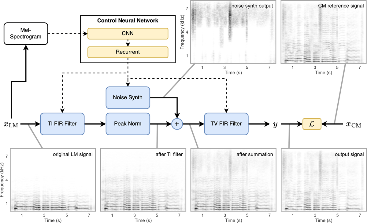
Figure 5
Architecture of the DDSP-based baseline system. Blue color is used for differentiable DSP building blocks, yellow color for NN building blocks with learnable parameters, and white color for fixed pre-processing steps. Control parameter flow is denoted with dashed line arrows, while solid lines indicate flow of audio signals. The spectrograms show signal content at the indicated position in the signal flow diagram. The shown example uses an excerpt from the LM-B signal of song AA T5 as the input signal xLM and a corresponding model trained with the OF scenario (see Section 6).
The parameters for these building blocks are provided by a control NN consisting of a convolutional neural network (CNN) with residual connections (ResNet, He et al. 2016) that receives a mel-spectrogram of the complete xLM as input. As the actual audio processing is done frame-wise in the time domain, a subsequent recurrent neural network directly outputs the parameters for the DSP building blocks at each frame, while accounting for long-term dependencies between frames. The time-invariant FIR filter uses only the last recurrent network output. For the TI FIR and the TV FIR filters, the control parameters are given as magnitudes in 64 linearly-spaced frequency bands, from which a linear-phase FIR filter is designed with an interpolation strategy, as proposed by Engel et al. (2020). Similarly, the Noise Synth uses randomly generated white noise, equalized by a filter whose magnitude response is prescribed by only 10 bands. Here, the reduced number of bands keeps the Noise Synth from producing narrow-band, quasi-harmonic noise sounds, which may improve the performance in terms of , but can lead to audible artifacts in the output audio. With this DSP processing pipeline, the model is guaranteed to retain the F0 that is present in xLM.
5.3 Implementation Details
We process audio with a sampling rate of 16 kHz and a frame size of 320 samples (resulting in a frame rate of 50 Hz). The input mel-spectrogram to the control NN with 64 frequency bands is calculated via an STFT using the Hann window of length 2048 samples and hop size 320 samples, resulting in the same number of frames as the time-domain processing. The time-varying control parameters of the TV filter and the Noise Synth are also updated at this rate. Therefore, this hyper-parameter influences the temporal resolution of the synthesis and thus the reconstruction quality. In initial experiments, we did not observe improvements from increasing the frame rate. Using lower rates may reduce training and inference times, while producing lower quality output signals. The TI, TV and Noise Synth filters are designed using linear interpolation of the magnitudes to obtain a linear-phase filter of length 320 samples. Filters are applied using FFT convolution and overlap-add between successive frames. The specific architectures for the CNN and recurrent parts are adapted from the original DDSP code base and we also use the multi-scale spectral loss function with their proposed configuration. During training, we use random excerpts from the respective training set (cf. Section 6) of four seconds length and train the model for 40,000 steps. Our metric between y and xCM is the multi-scale spectrogram loss, using the same parameters as introduced by Engel et al. (2020).
6. Experiments
In this section, we evaluate our baseline model with regard to its suitability for LM-SVR, using training data from LM-SSD. In the experiments, we use only takes without guitar crosstalk on the CM microphone (C0 condition, see Section 4.2) and train separate models for LM-A and LM-B inputs, respectively. To illustrate how the dataset can be split in different ways, we define three training scenarios, corresponding to increasing difficulty of the LM-SVR task:
Overfitting (OF): The model is trained on all six C0 takes of a single singer (from three songs) and evaluated on a take that is part of the training set. While this is not a realistic use case for the system, these results demonstrate an “upper bound” on the reconstruction quality that our baseline can achieve.
Different Take (DT): Here, the evaluation take is excluded from the training set, resulting in five training takes for each singer. Since LM-SSD contains multiple takes per song, the model has seen a different take of the evaluation song during training.
Different Song (DS): All takes of the evaluation song are excluded from the training set, resulting in four training takes. This is the most challenging scenario we consider, as the notes and words sung in the evaluation recording have not been seen during training.
A complete training run is done for each of these scenarios as described in Section 5.3. To keep the model in our illustrative example small and maintainable, we restrict the training scenarios to a separate model for each singer and LM type.
6.1 Evaluation
As an objective measure for the reconstruction quality of our baseline model, we use the Fréchet Audio Distance (FAD, Kilgour et al. 2019) between the CM signal and the reconstruction results. The FAD is based on the distance between learned general-purpose embeddings of the audio signals and we use the originally proposed VGGish (Hershey et al., 2017) embeddings for our evaluation. Since this embedding distance is independent of the exact waveform shape and has been shown to correlate with human perception, it is more suitable for our experimental setup than for example the signal-to-distortion ratio (SDR, Vincent et al. 2006), which requires a direct linear relationship between the compared signals. Beyond OF, DT, and DS, we include the conditions LM (for the unaltered LM signal) and NA (a naive reconstruction approach where the LM signal is filtered with the inverse of the RTF between the LM and CM microphones) in the comparisons. Using LM-A as the input signal, we obtain an average FAD of 0.76 for OF, 1.29 for DT, 1.51 for DS, 9.83 for LM, and 6.17 for NA (with LM-B: 0.77 for OF, 0.90 for DT, 1.17 for DS, 8.56 for LM, and 9.28 for NA) over a test set consisting of the eight songs in Table 3. These results indicate that the baseline model generally is able to reconstruct some perceptually relevant characteristics that are present in the CM signal but not in the LM inputs.
Table 3
Word error rate (WER) of lyrics transcription with the Whisper (Radford et al., 2022) medium model for a selection of songs from LM-SSD. Song DL uses the dedicated German Whisper model.
| WER (%) | ||||||
|---|---|---|---|---|---|---|
| SONG | SINGER | CM | LM | OF | DT | DS |
| AA | 1M | 1.83 | 72.56 | 1.83 | 22.56 | 20.73 |
| TS | 1M | 2.82 | 31.69 | 2.82 | 24.65 | 33.10 |
| DL | 2M | 2.16 | 10.81 | 2.70 | 5.95 | 7.03 |
| BB | 2M | 7.40 | 11.25 | 9.65 | 11.90 | 21.22 |
| SG | 3F | 3.70 | 11.11 | 5.76 | 11.11 | 57.61 |
| OC | 3F | 3.31 | 84.30 | 4.96 | 12.40 | 58.68 |
| CC | 4F | 0.49 | 92.65 | 0.49 | 29.41 | 91.67 |
| LL | 4F | 1.98 | 85.71 | 1.98 | 15.87 | 69.44 |
| Average | 3.27 | 49.05 | 4.25 | 15.89 | 46.13 | |
In order to assess the subjective quality of the reconstructions, also incorporating perceptual issues like lyrics intellegibility, which the FAD does not account for, we conducted a listening test comparing the six different conditions from above using a multi-stimulus test with hidden reference (denoted HR). In an online experiment using the WebMUSHRA interface (Schoeffler et al., 2018), participants were presented the reference (the original CM signals without crosstalk from LM-SSD) and asked to rate the other six stimuli (including HR) relative to that with respect to the overall perceived quality. All signals were played back with 16 kHz sampling rate and presented in mono via headphones. Rating was done on a continuous scale from 0 – 100, where 100 should be used for a signal that is indistinguishable from the reference and 0 should be used for a signal with subjectively bad quality. Participants were encouraged to make use of the whole scale in the test instructions. The test comprised 24 trials in random order using signals with a length between 6 and 10 seconds from all four singers and the different LM types. In total, 11 participants completed the test, two of which were excluded from our analysis as they did not consistently (in more than 85% of trials) rate HR with at least 90 points.
The results are presented in Figure 6, where the responses are split by singer identity. Generally, the training scenarios were rated in order of their difficulty level, where OF reached a mean score of 76, DT of 65, and DS of 49. This is in line with the occurrence of more artifacts like slurred consonants, particularly with the DS scenario,5 which, according to comments from some participants, impaired text intelligibility in the excerpts. All training scenarios reach better mean scores than the LM signal (17). The NA condition (mean score of 14) was not rated higher than the LM signal, possibly due to amplified noise. The stimuli with female singers (3F and 4F) tend to be rated slightly lower than male voice signals (mean score 50 vs. 57 over all stimuli). This discrepancy could follow from a lower F0 for males, which results in more partials in the sensitive frequency range of the LMs. However, these differences do not seem to be ameliorated by our baseline model.
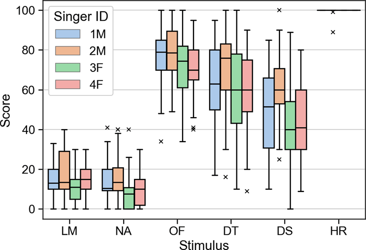
Figure 6
Listening test results according to stimulus and singer ID. LM: Larynx Microphone; NA: Naive Approach (linear filtering); OF, DT, DS: Overfitting, Different Take, and Different Song training scenarios; HR: Hidden Reference (CM signal).
6.2 Downstream Task: Lyrics Transcription
We consider lyrics transcription as an exemplary downstream task where LM-SVR may improve the performance of approaches that are optimized for high-quality singing recordings. In particular, we use Whisper (Radford et al., 2022), a state-of-the-art data-driven speech transcription system with a publicly available model that is pre-trained on a very large dataset. Even though it is not explicitly trained for the transcription of lyrics (see also Zhuo et al. 2023), it yields good results transcribing the singing voice from the CM signals in LM-SSD with a word error rate (WER) of 3.27% on average. For the LM signals, however, it yields a worse WER on average (49.05%) and a larger variance between songs, possibly because the model relies on features from full-band, high-quality speech recordings, which are largely lacking in the LM signals for some recordings. As retraining such a black box system with LM signals is not feasible, we explore how our LM-SVR baseline can improve transcription results, where a better performance would indicate that our model is able to reconstruct relevant characteristics of the singing voice signal. Detailed results for a selection of songs are presented in Table 3. The OF scenario (4.25% WER on average) reaches a similar performance to CM. Notably, the results with the DS scenario are sometimes inferior to the LM transcription (songs TS, BB, and SG in particular). While some errors are due to inconsistent spelling in the transcriptions (e.g., “supergirl” vs. “super girl”), these results indicate some unnatural distortion of formants and consonants in the model output when trained with the DS scenario. This may inspire future work on LM-SVR which can benefit from our dataset and the introduction of objective evaluation tasks like lyrics transcription.
7. Outlook & Conclusions
In this paper, we introduced LM-SVR as a novel MIR task. We publish LM-SSD, a dataset with LM and CM recordings of pop music with singer-songwriter instrumentation, and used these recordings to characterize typical LM signals. Furthermore, we evaluated a DDSP baseline for LM-SVR and showed that a model trained with LM-SSD has the potential to improve the subjective quality of LM singing voice recordings, as well as their usability for the downstream task of lyrics transcription, while preserving expressive intonation from the original recording.
Appendices
A. LM Signal Characterization
Let be the STFT time-frequency representations of two simultaneously recorded CM and LM signals of equal length, calculated using a Hann window with window size N, resulting in K frequency bins, and hop size H, resulting in M time frames. Furthermore, with ◦ denoting element-wise multiplication, we can define
as the frame-wise power spectrum of the CM signal and the LM signal, and the frame-wise cross-power spectrum between CM and LM signal, respectively.
A.1 Relative Transfer Function
Without access to the true relative transfer function (RTF) an unbiased estimate between CM and LM (Gannot et al., 2001, Eq. 31) can be calculated with
where {∙}M denotes taking the arithmetic mean over the M time frames. For the calculations in Figure 3, we use N = 32768 and H = 8192, with the signals at a sampling rate of 44.1 kHz. The RTFs are smoothed along the frequency axis with a Hann window of size 47 (a bandwidth of approx. 63 Hz).
A.2 Coherence
The frequency-dependent coherence estimate is given by
where is the element-wise complex conjugate of χ (Kates, 1992). For Figure 4, we use the same STFT parameters and smoothing as for the RTF. Choosing a large N and smoothing along the frequency axis contribute to a reduction of bias and variance, respectively, in the coherence estimate. Note that the naturally occurring time delay between CM and LM signals is small enough to have no relevant influence on the estimates.
Notes
[2] cf. for example Song BB on the accompanying website for a qualitative comparison of the different distortions in T1 (LM-A) and T4 (LM-B).
Acknowledgements
We would like to thank the musicians for their contribution to the dataset and Daniel Vollmer for his help with the LMs. The International Audio Laboratories Erlangen are a joint institution of the Friedrich-Alexander-Universität Erlangen-Nürnberg (FAU) and Fraunhofer Institute for Integrated Circuits IIS.
Funding Information
This work was funded by the Deutsche Forschungs-gemeinschaft (DFG, German Research Foundation) under Grant No. 401198673 (MU 2686/13-2).
Competing Interests
Meinard Müller is a Co-editor-in-Chief of the Transactions of the International Society for Music Information Retrieval. He was removed completely from all editorial decisions. The authors have no other competing interests to declare.
Author Contributions
Simon Schwär was main contributor to writing the article, creating the dataset, analysing signals, and running experiments. Michael Krause co-developed the baseline model and contributed to writing the article. Michael Fast helped recording the dataset, running baseline experiments, and conducting the listening test. Sebastian Rosenzweig co-developed the baseline model. Frank Scherbaum shared his expertise on LMs and provided the hardware. Meinard Müller supervised the work and contributed to writing the article.