

Figure 1
Differences between note alignments (left) and sequence alignments (right, e.g. produced by DTW). Note alignments can feature unaligned elements and the aligned note pairs are not guaranteed to be strictly ordered in time.
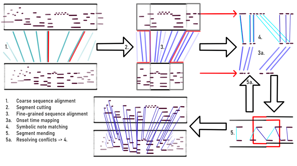
Figure 2
The steps involved in our proposed models: coarse sequence alignment, segmentation, fine-grained sequence alignment, note matching, and segment mending. For anchor point-based models treated in section 4, the first step is replaced by existing anchor points.
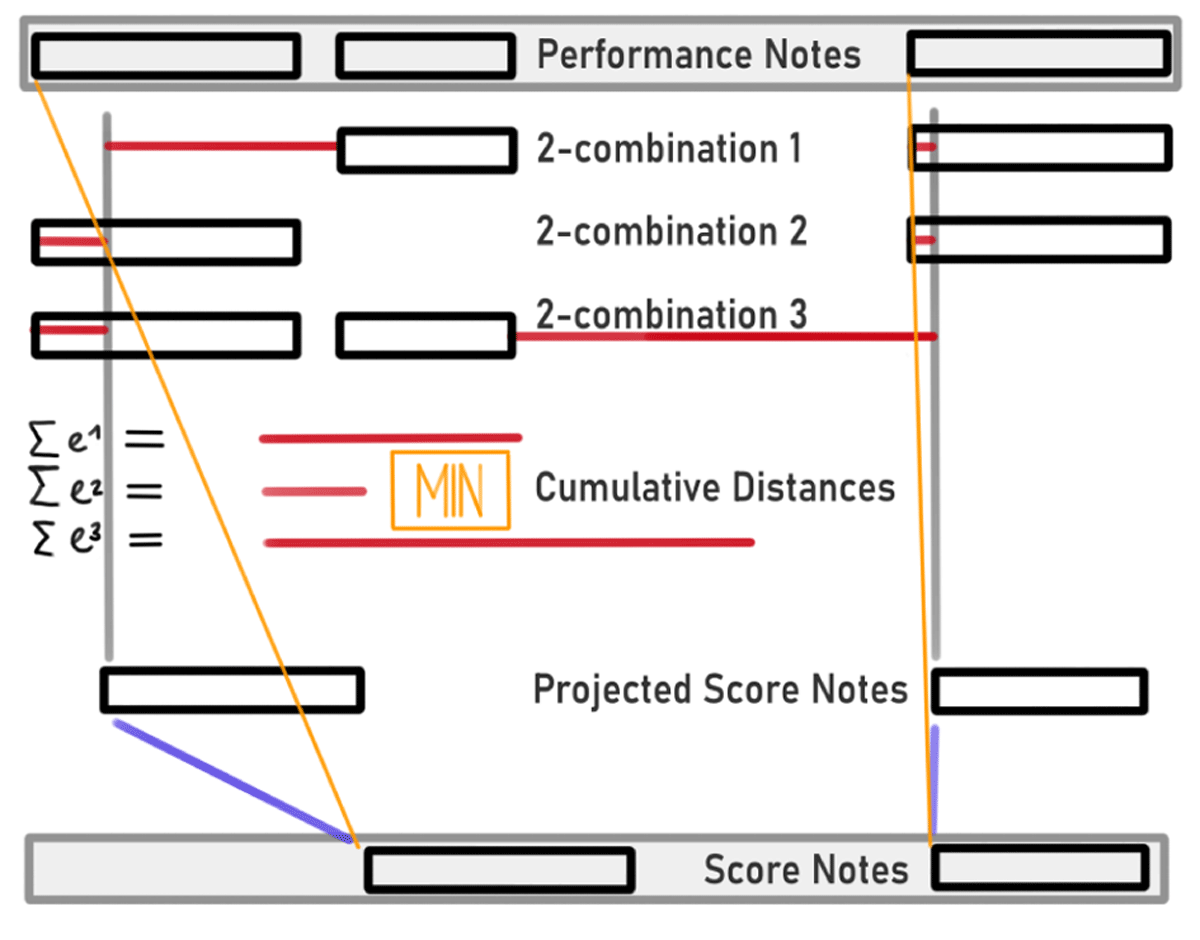
Figure 3
Pitch-wise symbolic note matching based on minimal cumulative distance between warped notes. Three performance notes (top row) are matched to two score notes (bottom row). First the score notes are projected to the performance time domain using a time mapping (blue lines). Second the distances of the projected score onsets from all 3C2 2-combinations of the three performance onsets are computed (rows two to four). Finally, the two performance notes minimizing the cumulative distance (red bars) are aligned to the score notes (yellow lines).
Table 1
Computation of precision and recall for a simple case of four notes; score notes sn1, sn2, and performance notes pn1, pn2. m() denotes a match, d() and i() deletions and insertions, respectively.
| VALUE | EXAMPLE |
|---|---|
| Prediction | m(sn1, pn1), m(sn2,pn2) |
| Ground truth: | d(sn1), i(pn1), m(sn2,pn2) |
| True Positive: | m(sn2, pn2) |
| False Positive: | m(sn1,pn1) |
| False Negative: | d(sn1), i(pn1) |
| Precision | 1/2 (= TP/(TP + FP)) |
| Recall | 1/3 (= TP/(TP + FN)) |
Table 2
Dataset-wise averaged F-Scores of each model. * Superscripts are not statistically different from Nakamura’s (α = 0.01).
| 4×22 | ZEILINGER | MAGALOFF | |
|---|---|---|---|
| hDTW+sym | 98.53 % | 97.98 %* | 94.57 %* |
| hNWTW+sym | 97.38 % | 95.07 %* | 90.91 % |
| Nakamura | 98.97 %* | 97.61 %* | 95.18 %* |
Table 3
Hyperparameter grid search values: window size refers to the search space of notes for the greedy algorithm, fuzziness refers to the amount of window overlap (see Section 4.1.1), metric refers to the local distance metric in the time warping algorithms, and γ refers to the gap penalty.
| METHOD | PARAMETERS | VALUES |
|---|---|---|
| Greedy | Window size: | 1, 3, 5 |
| Linear | Fuzziness: | 0.05n; n ∈ {1,…,20} |
| DTW | Fuzziness: | 0.05n; n ∈ {1,…,20} |
| Metric: | cos, Lp; p ∈ {1,2,4, ∞} | |
| NWTW | Fuzziness: | 0.05n; n ∈ {1,…,20} |
| Metric: | cos, Lp; p ∈ {1,2,4, ∞} | |
| γ: | 0.5, 1.0, 1.5 2.0, 2.5, 3.0 |
Table 4
Hyperparameters and F-measures of the best performing models on the tuning set.
| METHOD | HYPERPARAMETERS | F-MEASURE |
|---|---|---|
| Greedy | Window size: 3 | 95.43 % |
| Linear | Fuzziness: 0.95 | 98.71 % |
| DTW | Fuzziness: 0.65, L4-norm | 98.74 % |
| NWTW | Fuzziness: 0.8, γ: 0.5, Cosine | 98.75 % |
Table 5
Values with superscripts are statistically better (*) or worse (†) than Nakamura’s automatic alignment (α = 0.01), respectively. Bold indicates the best result (or results where the difference is not significant) for each resolution (beats, measures) and dataset.
| 4×22 | ZEILINGER | MAGALOFF | ||
|---|---|---|---|---|
| METHOD | F-MEASURE (IN %) | |||
| NAKAMURA | 98.97 | 97.61 | 95.18 | |
| Beats | Greedy | 99.28 | 98.09 | 95.68 |
| Linear | 99.87* | 99.67* | 98.87* | |
| DTW | 99.81* | 99.48* | 98.67* | |
| NWTW | 99.91* | 99.61* | 98.78* | |
| Measures | Greedy | 97.59† | 96.01 | 90.33† |
| Linear | 99.28 | 99.30* | 97.82* | |
| DTW | 99.31* | 98.88 | 97.66* | |
| NWTW | 99.63* | 99.25* | 97.88* | |
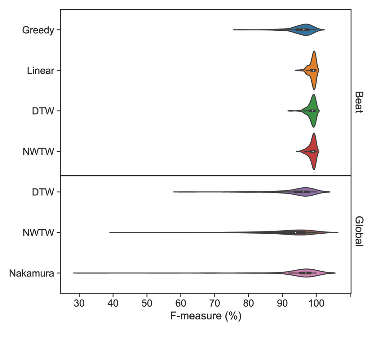
Figure 4
F-measure for models with global and beat level alignments. Results are reported on the Magaloff dataset.
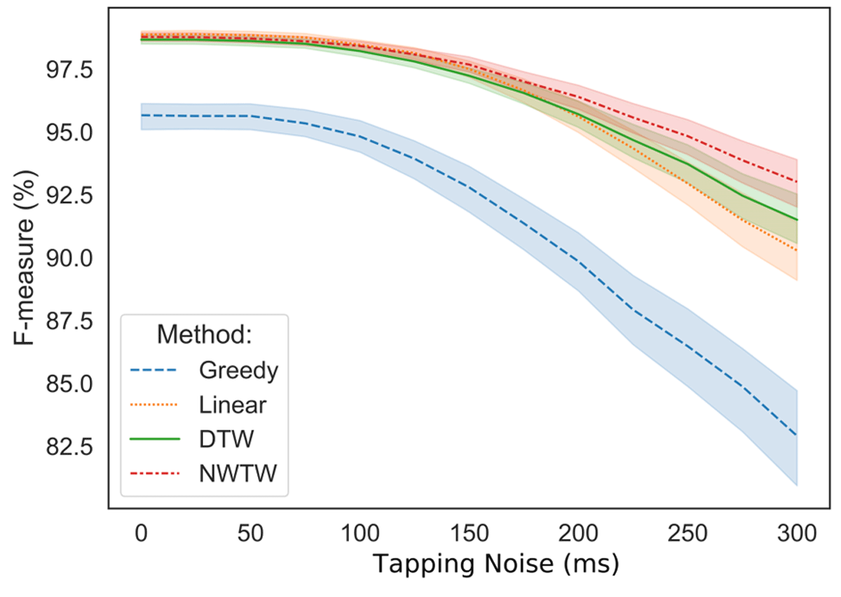
Figure 5
Effect of artificially added uniform noise on tapping annotations. Results are computed on the Magaloff dataset for beat-level alignments. The shaded areas indicate ±1 standard deviation from the mean.
Table 6
ASAP dataset statistics: S is the number of scores, P is the number of performances, S-Notes and P-Notes are number of notes in scores and performances, respectively, and Mins is the total duration of performances in minutes.
| COMPOSER | S | P | S-NOTES | P-NOTES | MINS |
|---|---|---|---|---|---|
| Bach | 59 | 169 | 117218 | 321688 | 387 |
| Balakirev | 1 | 10 | 16490 | 139608 | 87 |
| Beethoven | 63 | 271 | 431704 | 1668873 | 1761 |
| Brahms | 1 | 1 | 3514 | 1667 | 6 |
| Chopin | 36 | 289 | 236186 | 1410369 | 1257 |
| Debussy | 2 | 3 | 10800 | 14470 | 13 |
| Glinka | 1 | 2 | 4246 | 9074 | 10 |
| Haydn | 12 | 44 | 56230 | 190942 | 215 |
| Liszt | 17 | 121 | 181274 | 1192297 | 900 |
| Mozart | 6 | 16 | 33796 | 73927 | 78 |
| Prokofiev | 1 | 8 | 9438 | 38231 | 33 |
| Rachmaninoff | 4 | 8 | 13552 | 20941 | 30 |
| Ravel | 4 | 22 | 32248 | 108519 | 140 |
| Schubert | 15 | 62 | 134576 | 453464 | 499 |
| Schumann | 11 | 28 | 63593 | 122356 | 129 |
| Scriabin | 2 | 13 | 18342 | 145441 | 125 |
| All | 235 | 1067 | 1363207 | 5911867 | 5670 |
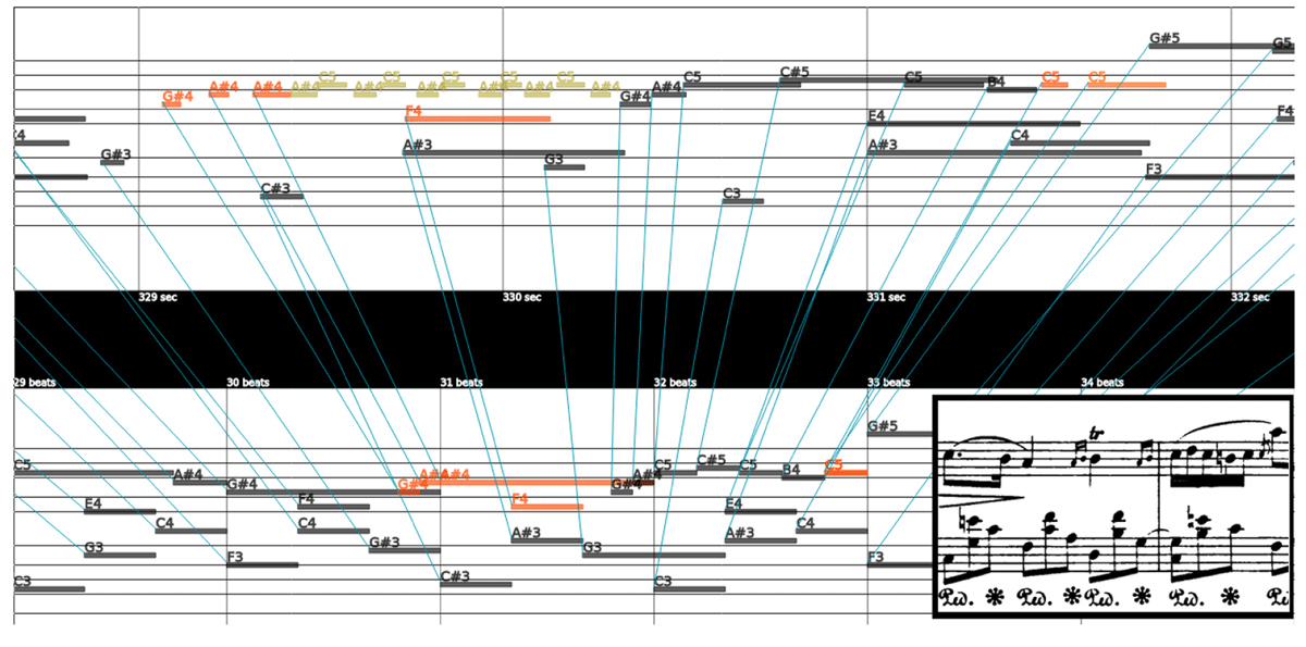
Figure 6
Parangonada visualization of an aligned excerpt of Chopin’s Nocturne Op. 32 No. 2, measures 8–9. The top piano roll represents the performance; the bottom piano roll the score. Lines connect notes aligned by automatic note alignment models. The score is added for clarity and is not part of the interface. Parangonada is not aware of pitch spelling; all black notes are displayed as ♯ even though the piece is in A♭ major.
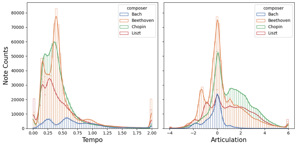
Figure 7
A histogram of the number of notes performed by composer and the performance statistics of those notes. Pieces from four composers were gathered: Chopin, Bach, Beethoven and Liszt. The left histogram plot shows onset-wise tempo in seconds per beat. The right plot shows a histogram of articulation expressed as a note-wise dimensionless logarithm of played duration divided by notated duration.
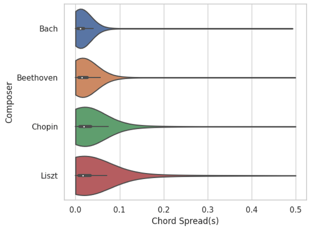
Figure 8
Chord spread distribution in seconds for four composers. Chord spread is defined for each chord as the maximal time interval between performance note onsets belonging to the chord. The white dot shows the median, the thick horizontal line the quartiles, and the thin horizontal line the 5- and 95-percentiles.
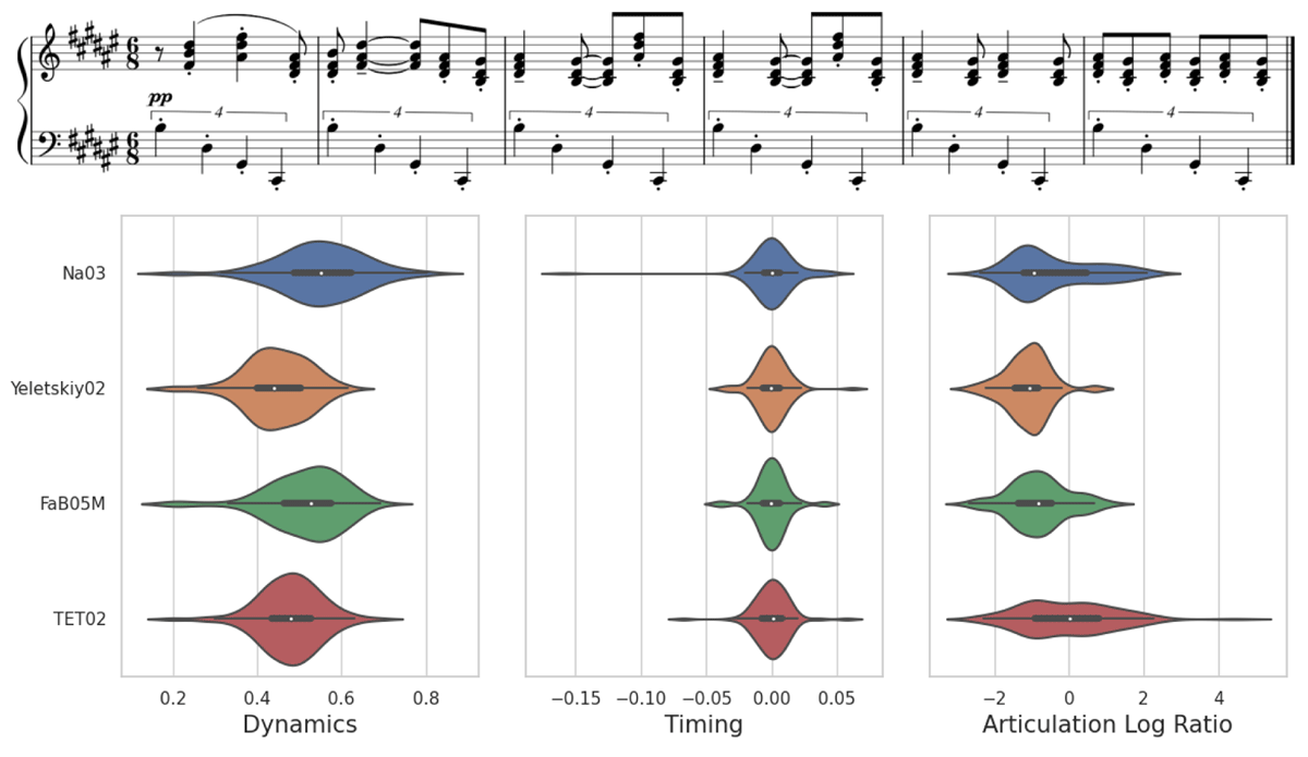
Figure 9
Performance statistics for four performers on the Scriabin Sonata No. 5, measures 47-52. Left: dynamics (MIDI velocity, normalized to (0,1)); middle: timing (how much onsets of chord notes deviate from their mean, in seconds); right: articulation (how staccato or legato the notes are played; see also Figure 7). The horizontal gray lines indicate quantiles; see also Figure 8.