
1 Introduction
Large annotated datasets are fundamental in many fields for data-driven models to be trained and evaluated, and the field of music information retrieval (MIR) is no exception. In MIR, some annotations, such as those for emotion and genre labels, can be produced relatively quickly and do not require the intervention of expert annotators, thus allowing large datasets to be crowd-sourced efficiently at scale. In contrast, other annotations require tedious and time-consuming manual work by people with significant musical expertise. This is the case for note alignment between a human MIDI performance and a musical score, since a music expert would need to manually pass through all notes in a music performance and mark a corresponding one in the score. This task is further complicated by possible player mistakes (e.g., missing or wrong notes) and score symbols such as mordents or trills, where a single score marking generates multiple (and sometimes an unspecified number of) performance notes. Since a piece of music can consist of thousands of notes, this process quickly becomes infeasible as the number of pieces to align increases, even with a dedicated graphical interface. Indeed, existing datasets with note alignments are of limited size: 88 MIDI performances in Vienna4x22 (Goebl, 1999) and 411 in CrestMuse-PEDB (Hashida et al., 2008). The MAPS dataset (Emiya et al., 2010) also contains note alignments, but does not contain real MIDI performances, only synthetic ones, simulated by randomly displacing the note positions to mimic the deviations introduced by the performers. Despite these difficulties, this type of alignment is fundamental for many MIR tasks such as performance-to-score music transcription (Nakamura et al., 2018), score following (Schwarz et al., 2004; Gu and Raphael, 2009; Arzt, 2016; Henkel et al., 2020), and expressive performance analysis (Cancino-Chacón et al., 2018; Lerch et al., 2020).
In this paper, we study several techniques to speed up the note-alignment process. They are then applied to the ASAP dataset (Foscarin et al., 2020), a large dataset of solo piano MIDI performances beat-aligned to MusicXML scores, to create (n)ASAP (= (note-)Aligned Scores And Performances) the largest publicly available note-aligned dataset, consisting of 1062 unique performances with a total of 7,275,074 annotated notes.
There exists a considerable body of literature on automatic techniques that produce note alignments, given a corresponding MIDI performance and a score (or two MIDI performances). They are typically based on dynamic programming algorithms, for example Dynamic Time Warping (DTW) (Dannenberg, 1984), Longest Common Subsequence (LCS) and “divide and conquer” (Chen et al., 2014), and Viterbi decoding on a Hidden Markov Model (HMM) (Nakamura et al., 2017; Gu and Raphael, 2009). We perform an evaluation of the available models on three manually annotated reference datasets, and propose a model based on a hierarchical variation of DTW that performs on par with the state-of-the-art model of Nakamura et al. (2017).
A closer look at the results of automatic techniques, however, reveals alignment mistakes that make them unsuited for the production of high-quality reliable annotations. In certain situations, typically when the performance greatly deviates from the musical score (e.g., major player mistakes), or when the interpretation of the musical score is not unique (e.g., trills and mordents), alignment errors are introduced, that often propagate through adjacent measures and create large sections of misalignments. Since it is not possible to know which pieces are incorrectly annotated, a tedious manual correction step would have to be performed on all data. While correction takes less time than a full manual note-level annotation, it would still require a considerable amount of time from music experts.
A solution that significantly improves the results of automatic alignments comes from other annotations that are already present in the ASAP dataset. It contains alignments at both the beat and the bar level. We employ such coarse annotations as anchor points to restrict the search space of the alignment algorithm. This effectively prevents cascading errors, as misalignments will not propagate beyond the next anchor point. We evaluate multiple algorithms on our three reference datasets to quantify the output quality that can be expected, and use the best performing algorithm to annotate the ASAP dataset. The produced note alignments are encoded in two formats: a tab-separated encoding chosen with a focus on ease of parsing and the match format (Foscarin et al., 2022) with a focus on inclusion of basic score information.
Together with the audio performances provided by the MAESTRO dataset (Hawthorne et al., 2019), our extended (n)ASAP dataset now includes performances as MIDI and audio files as well as scores as MusicXML files with uniquely identified notes, aligned at beat and note level, making it the largest and most complete resource for the myriad of MIR tasks that require fine-grained score information.
In addition to quantitative statistics on our reference datasets, we give qualitative measures of the accuracy of our alignment algorithm by investigating the results on all ASAP performances, and reporting on the alignment errors we encounter. For this manual inspection step, we develop a web-based note alignment visualization tool called Parangonada which we also make available.
Although the anchor point guided alignment algorithm was developed primarily to make use of ASAP’s existing annotations, it is still reusable in other contexts, since coarse-level temporal alignments are easier to produce, for example, by beat-tapping, and to manually correct. Moreover, our model was developed to deal flexibly with anchor points of any granularity, e.g., beat, measure, section, etc.
Overall, this paper has four main contributions:
the extension of the ASAP dataset with segment-constrained note alignments thus creating the largest fully note-aligned dataset (n)ASAP;
the design, evaluation, and publication of segment-constrained models for note alignment that flexibly leverage existing annotations and significantly outperform unconstrained automatic models;
the design, evaluation, and publication of automatic models for note alignment that produce results on par with the state of the art;
the introduction of Parangonada, a web-interface for visualizing and correcting alignment annotations.
Links to our dataset, models, and tools are provided in Section 7. After Section 2 which provides an overview of related work, we detail the contributions. The above contributions are presented in order of importance, however they build upon each other in inverse order so this paper is structured accordingly: Section 3 introduces note alignments and evaluates two automatic hierarchical time warping-based models for automatic note alignment. Section 4 augments the above models with existing annotations as anchor points and evaluates these segment-constrained models in a variety of settings. Section 5 details the note alignment of the ASAP dataset, including a discussion on its robustness and a presentation of various statistics, and finally Section 6 concludes the paper.
2 Related Work
This section provides a brief overview of models for symbolic score-to-performance alignment for Western classical music. We do not address here in depth the related task of music alignment in the audio domain, and interested readers can find such a discussion elsewhere (e.g., Wang, 2017; Arzt, 2016; Müller, 2015, chapter 3). Figure 1 contains an intuitive representation of the difference between note alignments and sequence alignments. Audio-to-score and audio-to-audio alignments match sequences of features. Note alignments match symbolically encoded notes. Although audio-to-audio alignment methods rely on similar sequence-to-sequence alignment techniques as some note-level midi-to-score alignment methods, there are fundamental differences between audio and symbolic representations. These differences lie mainly in the typical types of uncertainty and noise involved in the audio domain which are not present for symbolic representations, where entirely different problems can arise.
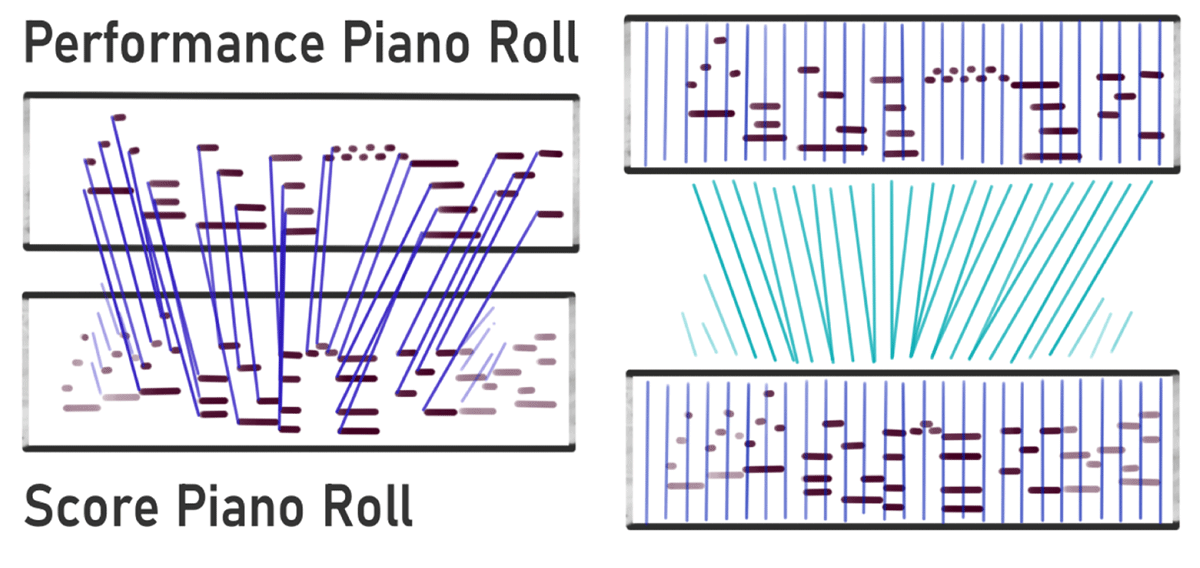
Figure 1
Differences between note alignments (left) and sequence alignments (right, e.g. produced by DTW). Note alignments can feature unaligned elements and the aligned note pairs are not guaranteed to be strictly ordered in time.
Furthermore, applicability of sequence-to-sequence alignment techniques to polyphonic symbolic note alignment is not straightforward; a central difficulty lies in finding a sequential representation for score chords that matches the played sequence of chord notes (Chen et al., 2014). Nevertheless, our work draws on two sequence-to-sequence alignment models for the preliminary alignment step of our models (see Section 3.1). A conceptually similar approach to our proposed model was introduced by Prätzlich et al. (2016), where multi-scale DTW was used for audio-to-audio alignment. This work was subsequently implemented in the Sync Toolbox (Müller et al., 2021). Another influence of audio-to-audio alignment techniques is the Needleman-Wunsch time warping algorithm (Grachten et al., 2013) which combines the Needleman-Wunsch algorithm (Needleman and Wunsch, 1970) with DTW. Furthermore, anchor point-based or segment-constrained approaches have been applied to audio-to-score alignment (Müller et al., 2004). Similar measure-wise constraints have been used in the generation of The Multimodal Schubert Winterreise Dataset (Weiß et al., 2021).
Models for symbolic music alignment date from the mid-1980s with pioneering work by Dannenberg (1984) and Vercoe (1984). They are commonly based on probabilistic sequential models like hidden Markov models (HMMs) or their derivatives (e.g., Schwarz et al., 2004; Gu and Raphael, 2009; Nakamura et al., 2015, 2017), or on dynamic programming algorithms such as dynamic time warping (DTW; e.g., Dannenberg, 1984) or Least Common Subsequence (LCS; e.g., Chen et al., 2014). Gingras and McAdams (2011) showed that the inclusion of additional features such as voice and tempo information can improve the quality of the alignments. State-of-the-art polyphonic note alignment models often bypass a pure sequence-to-sequence alignment step altogether. One of the most widely used automatic score-performance alignment tools is the one introduced by Nakamura et al. (2017), based on hierarchical HMMs. We use this model as state-of-the-art reference for evaluation. Nakamura et al.’s approach frames alignment as an alignment, error detection, and realignment process. First, they compute an alignment using a hierarchical HMM approach on chords and on chord notes. Second, difficult areas are identified using heuristics based on unaligned or erroneous notes in the first alignment. Lastly, an improved HMM-based realignment is computed on the difficult areas, this time split into two voices corresponding to left and right hand (assuming piano music).
In terms of datasets, there has been a recent effort to generate data through crowdsourcing (e.g., Weigl et al., 2019). A common way to collect alignments for audio performances is through reverse conducting (i.e., tapping) (Dixon and Goebl, 2002). This process marks some temporal positions in the audio files (usually corresponding to beats or downbeats) that can be mapped to score positions. See, for example, the work on the Mazurka project (Sapp, 2007), the CrestMusePEDB dataset (Hashida et al., 2017), and the Musical Themes Dataset (Zalkow et al., 2020).
In this paper, we focus on the ASAP dataset, which is not crowd-sourced but is the product of several iterative improvements and corresponding publications. The data was originally collected by the Yamaha Piano-e-competition (https://www.piano-e-competition.com). In 2018, the MAESTRO dataset compiling this data was released (Hawthorne et al., 2019). Jeong et al. (2019) augmented the data with MusicXML scores and an automatic alignment using the model by Nakamura et al. (2017). Based on this data, the ASAP dataset was released in 2020 (Foscarin et al., 2020), including improved scores and robust, manually checked and corrected beat alignments.
For an overview of datasets for symbolic score-to-performance alignment, we refer the reader to Cancino-Chacón et al. (2018); Lerch et al. (2020). For a more in-depth discussion on the complexity of preparing datasets of performances aligned to their scores, see Goebl et al. (2008).
3 Automatic Note Alignment
In this section, we discuss the use of automatic models to generate note alignments. Note alignments match individual notes in a performance to those on a score. Unlike alignments in audio files, which typically map each time point to at least one reference time point, note alignments match symbolic elements and can feature unaligned elements (see Figure 1). We encode note alignments as a list of note ID tuples. This note alignment definition is independent of encoding, i.e., MIDI files can be note aligned to other MIDI files just as sheet music scores can be note aligned to other scores. To facilitate the presentation in this work, we assume note alignment between (sheet music) scores and MIDI performances and refer to the corresponding notes as such. Each note can be matched (the tuple combines a score note and a performance note), deleted (a tuple of an omitted score note and an “deletion” keyword) or inserted (a tuple of an “insertion” keyword and an extra performance note). This setting does not handle embellishments with unspecified note number and pitch (e.g., mordents and trills) separately, but rather classifies their notes as insertions. Note that while matched notes with different pitches could in principle be accepted, none of our models produces such alignments nor does the ground truth contain such matches.
To automatically generate note alignments we develop a class of models for note alignment based on two hierarchical steps of sequence alignment followed by a combinatorial optimization step to align notes. This class builds upon several algorithms, most notably sequence alignment techniques, discussed in Section 3.1, and symbolic note matching, discussed in Section 3.2. In the following (Section 3.3), we derive a class of hierarchical note alignment models from these algorithms. Figure 2 presents an overview of the steps in our proposed models. We evaluate these models with two versions of dynamic time warping against the state-of-the-art model by Nakamura et al. (2017) on three datasets of robust hand-corrected note alignments.
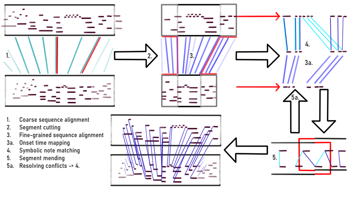
Figure 2
The steps involved in our proposed models: coarse sequence alignment, segmentation, fine-grained sequence alignment, note matching, and segment mending. For anchor point-based models treated in section 4, the first step is replaced by existing anchor points.
3.1 Sequence Alignment Algorithms
For sequence alignment we rely on two commonly used time warping algorithms. The algorithms are adapted to compute a sequence alignment between piano rolls (88×N binary matrices) of the score and performance. The output of each algorithm is a mapping between score and performance times.
3.1.1 Dynamic Time Warping
We use (vanilla) DTW to compute a time mapping between a score and a performance. Our DTW takes piano roll representations of score and performance as inputs, and optimizes a monotonically increasing match between two vector-valued sequences (in this case, the piano roll slices) using a local distance metric. The result is returned as an optimal path that matches piano roll slices of the performance with corresponding slices of the score with minimal cumulative distance. The piano rolls are generated with a granularity of 16 samples per beat and per second, for score and performance, respectively. For a more detailed description of the DTW, see Müller (2015, chapter 3).
3.1.2 Needleman-Wunsch Time Warping
Similar to DTW, Needleman-Wunsch time warping (NWTW; Needleman and Wunsch, 1970) is a dynamic programming algorithm that we use to compute a time mapping between a score and its performance. Originally proposed as a way to deal with structural differences between music performances, this algorithm combines the Needleman-Wunsch (NW) algorithm and DTW. It allows the matching of multiple elements of one sequence to a single element in the other sequence (as in DTW), while still allowing the possibility of a “jump” (as in NW), which is controlled by a constant parameter referred to as the gap penalty (γ). As in the DTW described above, we use piano roll representations of the score and performance information as inputs for the NWTW. For a technical description of NWTW, we refer the reader to Grachten et al. (2013).
3.2 Symbolic Note Processing
Symbolic note processing derives note alignments from sequence alignments. We model note alignment as a combinatorial optimization problem. First, the score and performance notes are separated into sequences by pitch. Second, we compute an approximate performance onset time for all score notes of a given pitch using the time mapping given by the sequence alignment. This time mapping is shown in the bottom (blue line) of Figure 3 as well as in the top right (step 4) of Figure 2. The time mapping is derived from a fine-grained time warping (step 3) or linear interpolation between the window limits. Lastly, as the number of notes in either sequence is not guaranteed to be the same, we use a combinatorial optimization step to determine which notes are insertions or deletions. In the following, we denote the set of (projected) score note onsets as S and the set of performance note onsets P. This is computed separately for each segment and pitch; the window and pitch indices are omitted for readability. Assuming without loss of generality that the number of score notes is not greater than the number of performance notes (|P|≥|S|), the last step is formalized as follows:
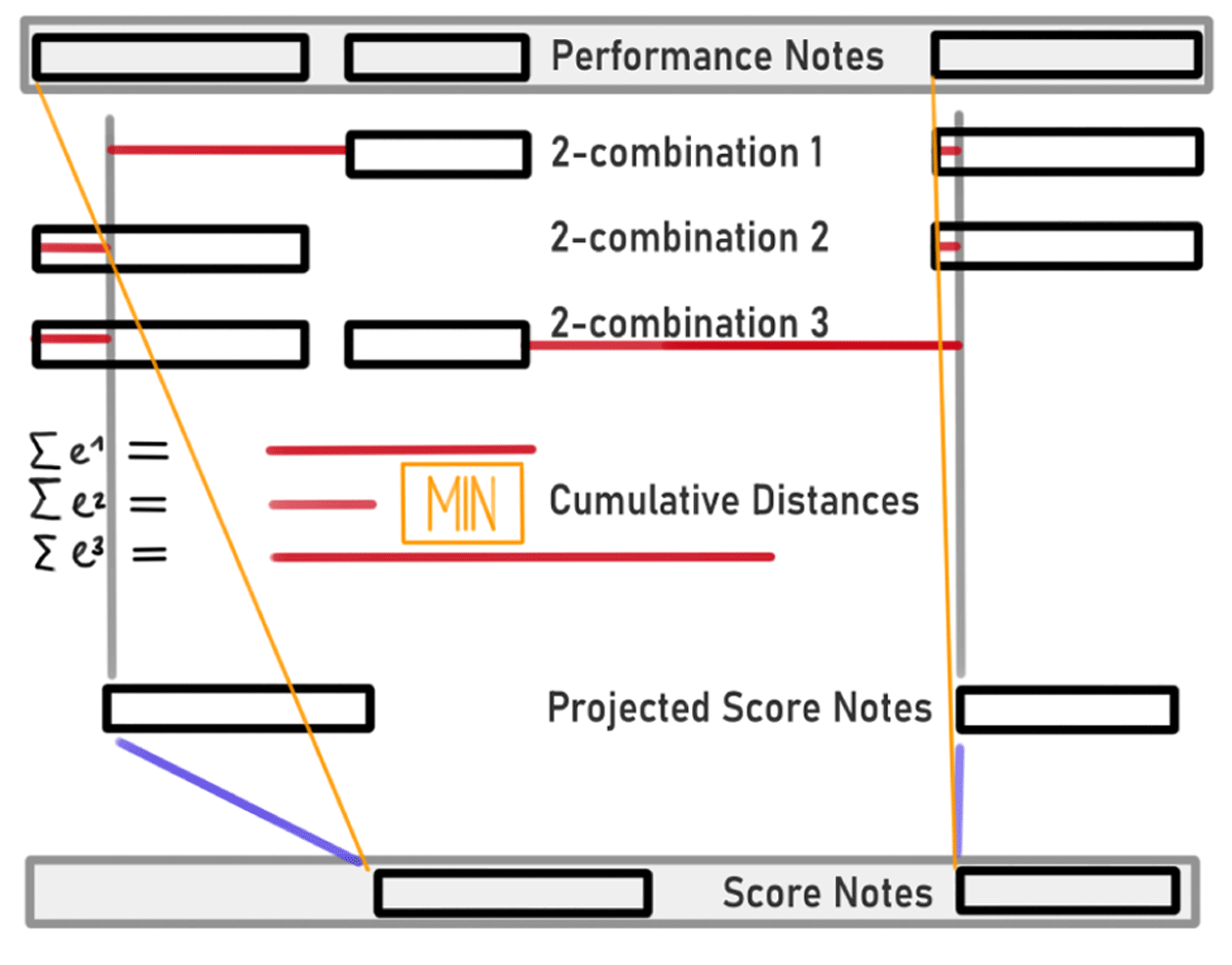
Figure 3
Pitch-wise symbolic note matching based on minimal cumulative distance between warped notes. Three performance notes (top row) are matched to two score notes (bottom row). First the score notes are projected to the performance time domain using a time mapping (blue lines). Second the distances of the projected score onsets from all 3C2 2-combinations of the three performance onsets are computed (rows two to four). Finally, the two performance notes minimizing the cumulative distance (red bars) are aligned to the score notes (yellow lines).
where the minimum is taken over all i ϵ I the |S|-combinations of performance onsets P, i.e., all subsets of P with cardinality |S| and distinct members. The number of combinations is thus given by |P|C|S|or equivalently by the binomial coefficient of |P| over |S|. Sk and refer to the onset position of the kth note in S and the kth note in the ith combination of notes from P, respectively, and i* refers to the combination that minimizes their pairwise distance.
The top of Figure 3 illustrates this optimization over all 2-combinations of three performance notes. Note that this algorithm is unable to discern both insertions and deletions in the same window, as it aligns the maximal number of notes available. This implicitly favors matches over insertions and deletions. However, the algorithm is symmetric with respect to insertions and deletions, i.e., if |P|>|S| unaligned notes are insertions and if |P|<|S| unaligned notes are deletions. For long sequences with many insertions or deletions, the optimization loop over all possible combinations of indices becomes computationally expensive.
3.3 A Hierarchical Model
We derive a class of hierarchical, automatic note alignment models from the aforementioned algorithms. The symbolic note matcher (3.2) is only suitable for short sequences due to its combinatorial bottleneck and its inability to detect both insertions and deletions of the same pitch in the same window. In order to circumvent these problems for a default case where the single window would cover the entirety of both score and performance, we divide the sequence alignment in two hieararchical steps. In a first step, a preliminary, coarse sequence matching is computed between the score and performance piano rolls. The score is cut into segments every four beats, and the cut times are mapped approximately to the performance using the computed sequence alignment. The segment length of four beats is a tuneable hyperparameter, and is not related to the musical material or its time signatures. The performance is then cut into segments at the corresponding times. These segments are then used as inputs to the algorithms discussed above: a fine-grained sequence alignment aligns the local piano roll segments and the symbolic note processor derives an optimal note match. See Figure 2 for an overview of our proposed model class. The technical details of segment cutting and mending, as well as resolution of alignment conflicts (Figure steps 3, 5, and 5a) are presented in Section 4. This two-step sequence matching approach is conceptually similar to multi-scale DTW as presented by Prätzlich et al. (2016).
3.4 Experiments and Datasets
To compare our automatic model against the state of the art, we evaluate three models on three large datasets. The models are the reference model by Nakamura et al., our proposed DTW-based hierarchical note alignment, and our proposed Needleman-Wunsch time warping based hierarchical note alignment. Note that in the second and third models, both coarse and fine-grained sequence alignment is computed by the same version of time warping, respectively. We refer to the models as Nakamura, hDTW+sym, and hNWTW+sym, respectively.
For the evaluation of the proposed models, we use three datasets of high-quality, manually note-aligned piano performances, all of them recorded on computer-controlled Bösendorfer grand pianos. The Magaloff dataset (Flossmann et al., 2010) consists of (nearly) all solo piano works by Chopin, performed by Nikita Magaloff. This dataset consists of more than 150 pieces, for a total of more than 300k performed notes (ca. ten hours of music). The Zeilinger dataset (Cancino-Chacón et al., 2017) consists of nine full Beethoven piano sonatas performed by Clemens Zeilinger. This dataset contains 29 performances (each movement is counted as a separate piece), with more than 70k performed notes (ca. three hours of music). Finally, the Vienna 4×22 dataset (Goebl, 1999) consists of four pieces/excerpts (two by Chopin, one by Mozart, one by Schubert) performed by 22 pianists. This dataset contains 88 performances, with more than 40k performed notes (ca. two hours of music).
3.5 Results
Throughout this section and in subsequent experimental results, we report the predictive quality of the models as F-measures, averaged across each dataset. The F-measure refers to the harmonic mean of precision and recall of the predicted performance-wise alignment. A predicted match is counted as a true positive only if the notes are matched in the ground truth alignment. A predicted insertion or deletion note is counted as true positive if the note is marked as an insertion or a deletion in the ground truth, respectively.
A false positive is a predicted note label that isn’t in the ground truth, a false negative is a ground truth note label that isn’t predicted. All notes have a predicted label as well as a ground truth label, so false negatives always correspond to false positives, and vice versa, albeit not necessarily the same number.
We illustrate this adapted F-measure with an example in Table 1: A misalignment of two notes that are unaligned in the ground truth creates one false positive match and two false negatives: a deletion and an insertion. True negatives do not exist in this setting. Note that this measure does not discriminate the types of errors: mismatches, false matches, and false insertions or deletions.
Table 1
Computation of precision and recall for a simple case of four notes; score notes sn1, sn2, and performance notes pn1, pn2. m() denotes a match, d() and i() deletions and insertions, respectively.
| VALUE | EXAMPLE |
|---|---|
| Prediction | m(sn1, pn1), m(sn2,pn2) |
| Ground truth: | d(sn1), i(pn1), m(sn2,pn2) |
| True Positive: | m(sn2, pn2) |
| False Positive: | m(sn1,pn1) |
| False Negative: | d(sn1), i(pn1) |
| Precision | 1/2 (= TP/(TP + FP)) |
| Recall | 1/3 (= TP/(TP + FN)) |
Results of the model comparison are collected in Table 2. For the Vienna 4x22 and the Magaloff datasets, we found a statistical difference (α = 0.01) between the average F-measures of these models. This result was computed using the Friedman test (Field et al., 2012), a non-parametric alternative to repeated measures ANOVA, since the values of the F-measures violate the normality assumptions ANOVA requires. To test the pairwise differences between NWTW/DTW and Nakamura, we used Wilcoxon signed-rank tests with Bonferroni correction (Field et al., 2012). The results of these tests suggest that the hierarchical DTW model performs on par with Nakamura for both Zeilinger and Magaloff datasets (the ones with the most complex pieces).
4 Note Alignment from Anchor Points
While the models presented in the previous section perform well, they still encounter the same difficulties that previous automatic models have. For some pieces and performances, the coarse sequence alignment fails and large chunks of the resulting alignments are faulty and unreliable.
4.1 Anchor Points
In this section, we incorporate existing coarse annotations as anchor points into our models to restrict the search space of the alignment algorithm. Specifically, we replace the first coarse sequence alignment step by existing beat, measure, or any other anchor point annotations (see step one in Figure 2). Using a segmentation derived from these anchor points, local symbolic note matching is performed, augmented by fine-grained time warping information.
We present three experiments for note alignments based on anchor points to assess the effects of each part in the models. We first introduce a formal description of the anchor point based segmentation and add two simple baseline algorithms.
4.1.1 Segmentation
Anchor point alignments are not only more coarse, but also structurally different from note alignments. Anchor points are not symbolically encoded, but refer to perceptual markers (usually obtained by manually tapping beats or measures) in the performance time. For a given anchor point (Ai = (si, pi))—consisting of a beat position (si) in the score and its corresponding time (pi) in the performance—any note sufficiently close to the score anchor might fall on either side of the performance anchor. To mitigate this, we use overlapping score and performance windows (Wi = (Si, Pi)). The fuzziness (f) hyperparameter refers to the length of this overlap in beats. The windows are defined as follows:
where np and np refer to score and performance notes, respectively, and ci is the local tempo, i.e. the ratio of the performance interval divided by the score interval between two anchor points.
The window overlaps lead to multiple—sometimes conflicting—symbolic note matches produced by window-wise models (Figure 2 bottom right illustrates two overlapping window-wise models with conflicts). While non-conflicting matches are straightforward to merge into a longer alignment, dealing with conflicting matches is more complex. We therefore propose an alignment merging algorithm that traverses the graph of both (or all) conflicting note annotations whenever conflicts (both conflicting matches as well as matches conflicting with insertions or deletions) are encountered. In Figure 2 this connected note graph would return the central five notes that cannot be unanimously matched. One of the score notes is a deletion, but the window-wise models disagree about which it is. The collected cluster of notes is matched again using a single call to the symbolic note processor (3.2, step 5a in Figure 2) given a linear time interpolation of the surrounding alignment anchor points. This process guarantees uniqueness and monotonicity per pitch sequence.
4.1.2 Baseline Algorithms
We add two baseline algorithms: one for sequence alignment (see 3.1), and one for symbolic note matching (see 3.2). Linear time interpolation refers to a locally linear time mapping between score and performance, that is obtained by linear interpolation of the anchor points anchor points). This serves as a linear baseline for the more sophisticated DTW and NWTW matching functions. Analogous linear time extrapolation is used in the computation of the overlapping extension of performance windows (see Equation (5) above).
As a simple baseline for the combinatorial symbolic note processor, we use a greedy algorithm. Greedy note alignment searches for the closest unmatched performance note of matching pitch for every score note and, if one is found, aligns them (Figure 2 top right, step four illustrates this behavior). Dark blue lines match notes using minimization over cumulative distance (after mapping to the same time line) where the light blue lines are added greedily, i.e., the first six performance notes are aligned to the first six score notes. The search is executed window-wise, where the number of performance windows before and after the main window is determined by a hyperparameter. Leftover score and performance notes are deletions and insertions, respectively. Greedy alignment is independent of local time warping and only works for suitably small windows; however, it is an important baseline for the beat anchor points.
4.1.3 Anchor Point Experiments
Overall, we define four model classes from the introduced algortihms: A Greedy model that uses greedy note matching in windows produced from anchor points without any call to sequence alignment, a Linear model that refers to linear time interpolation between anchor points to augment the combinatorial note processor, and DTW and NWTW models that use DTW and NWTW for time interpolation, respectively. In our experiments, we refer to the four main time warping and matching models as Greedy, Linear, DTW, and NWTW. All models with the exception of Greedy use linear interpolation for conflicting note alignments at overlaps. In order to compare our models, we design three experiments:
A tuning experiment (4.2) to find the best hyperparameters for each model class for note alignment based on anchor points.
A performance evaluation (4.3) on the four tuned models on the full datasets.
A robustness experiment (4.4) that tests the four tuned models against increasingly unreliable anchor point conditions.
All experiments are computed on the aforementioned datasets with known high-quality note alignment ground truth (see Section 3.4), from which we derive synthetic anchor points.
4.2 Tuning Experiments
This experiment consists of a hyperparameter grid search. The grid search is computed for the values in Table 3 under the beat-wise anchor points condition. To tune the hyperparameters of the models, we selected six pieces from the Magaloff and Zeilinger datasets, which present interesting difficulties for alignment systems (e.g., ornaments/trills, cross rhythms). The pieces are Nocturnes Op. 9 Nos. 1 and 2, Etude Op. 10 No. 11, Nocturne Op. 15 No. 2, the Barcarole Op. 60 by Chopin, and the third movement of the Sonata Op. 53 (Waldstein) by Beethoven. These pieces were only used for tuning the models and not included in the other two experiments on performance (4.3) and robustness (4.4).
Table 3
Hyperparameter grid search values: window size refers to the search space of notes for the greedy algorithm, fuzziness refers to the amount of window overlap (see Section 4.1.1), metric refers to the local distance metric in the time warping algorithms, and γ refers to the gap penalty.
| METHOD | PARAMETERS | VALUES |
|---|---|---|
| Greedy | Window size: | 1, 3, 5 |
| Linear | Fuzziness: | 0.05n; n ∈ {1,…,20} |
| DTW | Fuzziness: | 0.05n; n ∈ {1,…,20} |
| Metric: | cos, Lp; p ∈ {1,2,4, ∞} | |
| NWTW | Fuzziness: | 0.05n; n ∈ {1,…,20} |
| Metric: | cos, Lp; p ∈ {1,2,4, ∞} | |
| γ: | 0.5, 1.0, 1.5 2.0, 2.5, 3.0 |
The metrics tested are defined as follows:
The hyperparameters that resulted in the highest average F-measures for beat-wise anchor points are collected in Table 4. Note that for all conditions relying on time mappings, the optimal fuzziness is relatively high. However, shorter window overlaps sometimes result in similarly high F-measures, e.g., for the linear condition, an average F-measure of 98.60% was computed for fuzziness of 0.3. Fuzziness can be understood as a trade-off between matching more notes per window, but having more conflicting matches in post-processing. The different local metrics did not produce significantly different results for the DTW and NWTW conditions except for the L∞ norm. A similar grid search was performed for DTW and NWTW on the no anchor point condition, resulting in fuzziness and metric parameters of 4.0 and cosine distance. The larger fuzziness parameters can be attributed to the increased uncertainty of the DTW/NWTW-based anchor points.
4.3 Performance Experiments
This experiment evaluates the four tuned models on the full datasets. Two different synthetic anchor point conditions are computed: beat-wise and measure-wise.
Results of the model comparison on the different anchor point granularities are collected in Table 5. As a baseline, we again refer to the current state-of-the-art model proposed by Nakamura et al. (2017). To evaluate our proposed algorithms, we proceed in a similar way to the automatic model evaluation (Section 3.5) and compare these models to Nakamura’s with a Friedman test for each dataset and granularity (beat-wise/measure-wise). We find a statistical difference for all dataset and granularity combinations. We conducted Wilcoxon signed-rank tests with Bonferroni correction to test pairwise differences between each of the models (Greedy/Linear/DTW/NWTW) and Nakamura’s. As can be seen in Table 5, the results of these tests show improved results for almost all models that include anchor points and time mappings (values with * superscripts).
Table 5
Values with superscripts are statistically better (*) or worse (†) than Nakamura’s automatic alignment (α = 0.01), respectively. Bold indicates the best result (or results where the difference is not significant) for each resolution (beats, measures) and dataset.
| 4×22 | ZEILINGER | MAGALOFF | ||
|---|---|---|---|---|
| METHOD | F-MEASURE (IN %) | |||
| NAKAMURA | 98.97 | 97.61 | 95.18 | |
| Beats | Greedy | 99.28 | 98.09 | 95.68 |
| Linear | 99.87* | 99.67* | 98.87* | |
| DTW | 99.81* | 99.48* | 98.67* | |
| NWTW | 99.91* | 99.61* | 98.78* | |
| Measures | Greedy | 97.59† | 96.01 | 90.33† |
| Linear | 99.28 | 99.30* | 97.82* | |
| DTW | 99.31* | 98.88 | 97.66* | |
| NWTW | 99.63* | 99.25* | 97.88* | |
An unexpected result is the performance of the linear time interpolation in the beat-wise condition. We conjecture that due to the limited room for tempo variation within a single beat, the linear interpolation fits the true alignment well. NWTW and DTW on the other hand align windows of a beat extended by a considerable amount of overlap, which adds variability and uncertainty to these time mappings. For longer windows, time warping models profit from their advantage in flexibility over simple linear interpolation.
While the median F-measures are consistently high, even in the automatic setting, there are fewer and less extreme outliers for models that leverage anchor point information. Figure 4 illustrates this result per model as the F-measure distribution on the Magaloff dataset. One important practical question is whether it would be possible to identify these potentially difficult-to-align pieces beforehand and produce anchor points for only those pieces. We compute the Jaccard index (Levandowsky and Winter, 1971) to quantify the overlap between difficult-to-align pieces (with F-measure < 80%) for each pair of the automatic models. We find an average overlap of 16 %, with only one piece in common between all models. Since different automatic models fail on different pieces, the prediction of difficult-to-align pieces is clearly not trivial.
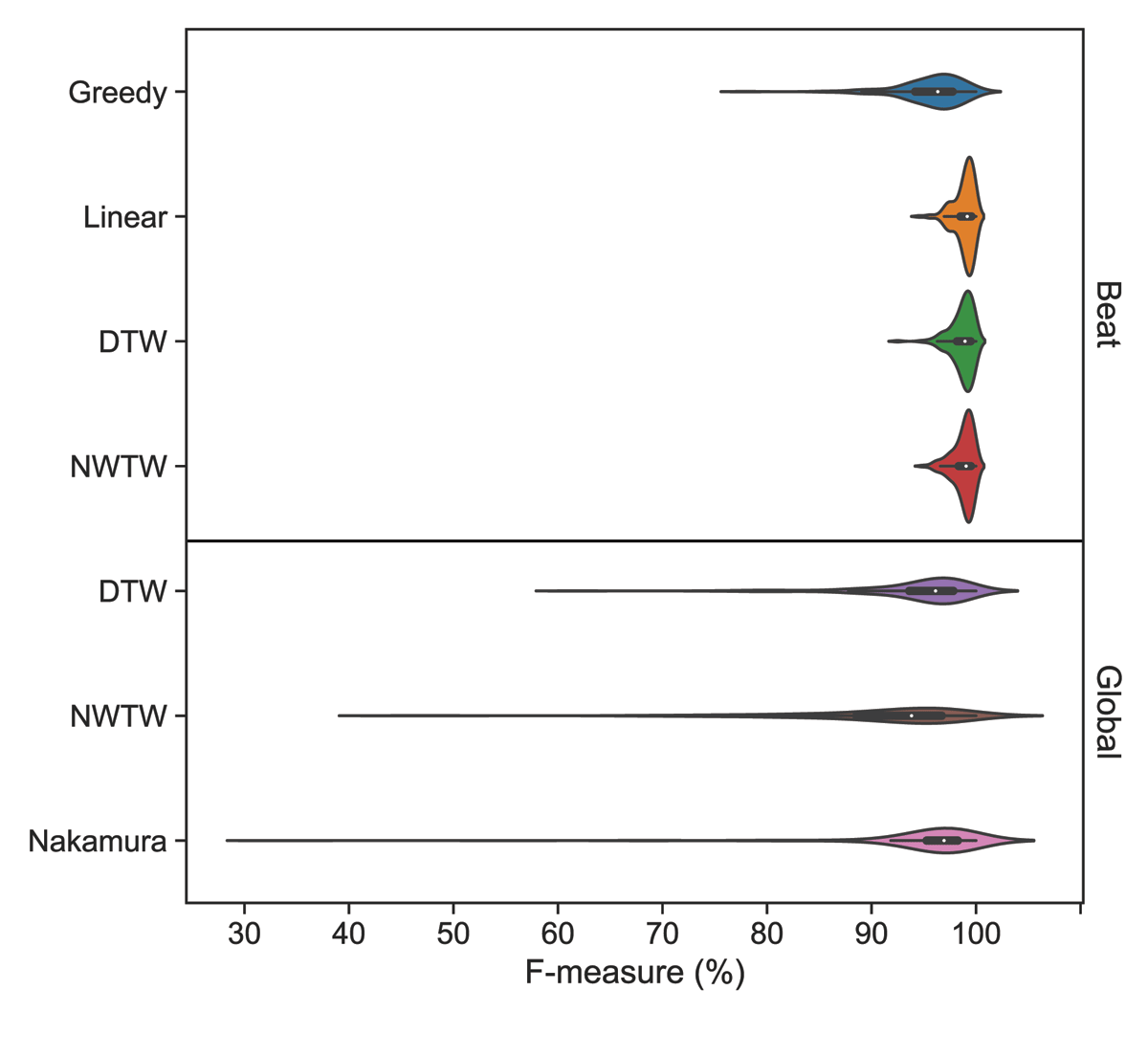
Figure 4
F-measure for models with global and beat level alignments. Results are reported on the Magaloff dataset.
4.4 Robustness Experiments
This experiment evaluates the robustness of the tuned models under increasingly unreliable anchor point conditions. Human annotations, especially when created by tapping along to a performance without cleaning the annotations, are subject to motor noise and other impressions. The introduced temporal deviations might throw the models off track. A robust model allows for large deviations without performance losses.
This is an important feature that allows human anchor point annotations to be created with minimal effort. We simulate errors and imprecision in tapping by adding noise to the performance anchors of the anchor points. Its effect on predictive quality is investigated for uniformly distributed noise between 0 and ±300 ms in increments of 25 ms.
The results of the robustness experiment are visualized in Figure 5. All models perform consistently for noise levels below ±100 ms, and degrade almost linearly for higher noise levels. At higher noise levels, the time mapping augmented models in general—and NWTW in particular—are shown to be more robust.
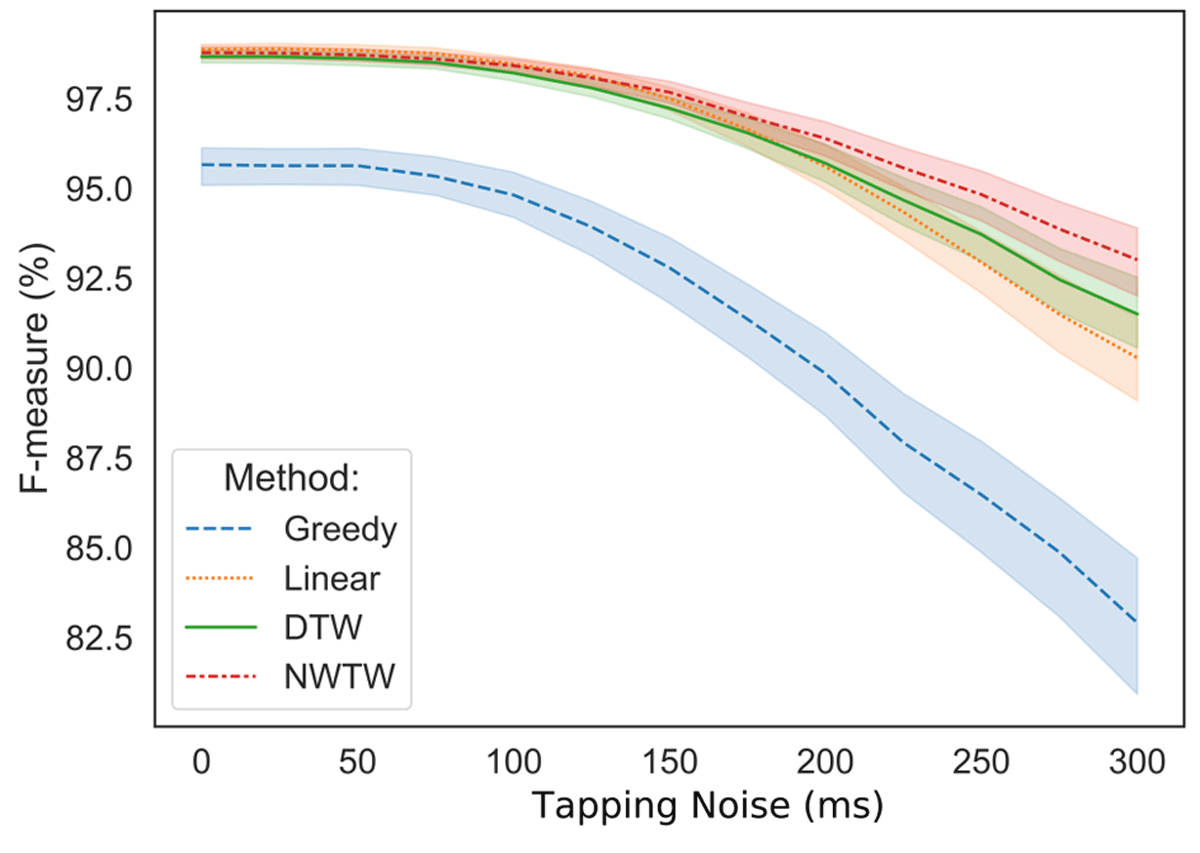
Figure 5
Effect of artificially added uniform noise on tapping annotations. Results are computed on the Magaloff dataset for beat-level alignments. The shaded areas indicate ±1 standard deviation from the mean.
For context, professional musicians can synchronize their playing with less than 20 ms errors (Goebl and Palmer, 2009). More closely related to our tapped anchor points, Gadermaier and Widmer (2019) estimate the distribution of beat-wise annotations of symphonic music, and find performance-wise median beat annotation standard deviations between 27 and 68 ms Our models are robust within these ranges of tapping noise.1
5 Alignment of the ASAP Dataset
As our main contribution, we produce reliable note alignments for the ASAP Dataset. ASAP is a large downbeat and beat aligned collection of symbolic scores (MusicXML files) and performances (MIDI files). As described in Section 2, this dataset was collected and refined in several iterations. It contains more than 1000 performances of over 200 pieces of common practice period solo piano music (see Table 6 for detailed numbers of dataset composition). The performances in the dataset are recorded on computer-controlled grand pianos during a piano performance competition. The performers of the Piano-E-Competition are adolescents or young adults playing highest-level piano competition repertoire.
Table 6
ASAP dataset statistics: S is the number of scores, P is the number of performances, S-Notes and P-Notes are number of notes in scores and performances, respectively, and Mins is the total duration of performances in minutes.
| COMPOSER | S | P | S-NOTES | P-NOTES | MINS |
|---|---|---|---|---|---|
| Bach | 59 | 169 | 117218 | 321688 | 387 |
| Balakirev | 1 | 10 | 16490 | 139608 | 87 |
| Beethoven | 63 | 271 | 431704 | 1668873 | 1761 |
| Brahms | 1 | 1 | 3514 | 1667 | 6 |
| Chopin | 36 | 289 | 236186 | 1410369 | 1257 |
| Debussy | 2 | 3 | 10800 | 14470 | 13 |
| Glinka | 1 | 2 | 4246 | 9074 | 10 |
| Haydn | 12 | 44 | 56230 | 190942 | 215 |
| Liszt | 17 | 121 | 181274 | 1192297 | 900 |
| Mozart | 6 | 16 | 33796 | 73927 | 78 |
| Prokofiev | 1 | 8 | 9438 | 38231 | 33 |
| Rachmaninoff | 4 | 8 | 13552 | 20941 | 30 |
| Ravel | 4 | 22 | 32248 | 108519 | 140 |
| Schubert | 15 | 62 | 134576 | 453464 | 499 |
| Schumann | 11 | 28 | 63593 | 122356 | 129 |
| Scriabin | 2 | 13 | 18342 | 145441 | 125 |
| All | 235 | 1067 | 1363207 | 5911867 | 5670 |
5.1 Alignment Encoding and Repetitions
One of the noteworthy differences that the change from beat-level (or sequential) alignments to note alignments engenders is the encoding of repetitions. In the original ASAP dataset, beats and downbeats are annotated for score and performance MIDI files. In the accompanying MusicXML score, the musical material of the score MIDI file is sometimes represented with a number of score navigation markers: repetitions, Codas, Segnos, Fines, etc. ASAP solves the possible mismatch between the implicitly notated musical material in the MusicXML and the played material in the MIDI scores by adding a “downbeats to score” mapping for each MIDI file. This mapping links each downbeat in a MIDI file with a measure in the MusicXML score. Whenever a score section is repeated, the downbeat counter jumps back to the start of the section, i.e., multiple downbeats can refer to the same measure in the score, one for each time it is played. For note alignments we chose a different approach to avoid the situation of having multiple performed notes aligned to the same score note. As a preprocessing step, we unfold the MusicXML scores to the played length by copying repeated sections and updating the IDs of the notes contained therein.
Given such an unfolded, longer score, we align the performance beats and downbeats to score positions using aforementioned downbeats to measure mapping. Once this alignment is computed, it serves as anchor points for the segment-constrained note alignment.
5.2 Technical Alignment Details
Note alignment was carried out using the best performing algorithm evaluated above on non-noisy input with beat alignments: linear interpolation with 0.95 window fuzziness. Notably, no dynamic time warping of any kind was used for the final note alignment. For each performance, we store two alignment files. One easy-to-parse tsv file that maps the notes in the MusicXML (by ID) to the notes in the MIDI performance (by track, channel, time, and pitch), including insertion and deletion for insertions and deletions, respectively. Secondly, we provide an alignment file for each performance in the more complete match file format (Foscarin et al., 2022). To make these alignments easy-to-use for future research, we add an ID field to each note in the MusicXML scores. This field does not impact users’ ability to parse them with any tool we tested (music21, MuseScore, and Finale). Note that the IDs in match and tsv alignments are derived from the IDs in the MusicXML score file, but suffixed by an integer corresponding to the repeat. E.g. n112-1 in an alignment file refers to the MusicXML note n112 played for the first time. If this note is repeated (i.e.it is in a section of the score that is repeated) its second occurrence is marked as n112-2. Functionality to process MusicXML, MIDI, and alignment files is publicly available in the Partitura Python library (Cancino-Chacón et al., 2022).
5.3 Manual Checks and Parangonada
The above model comparison indicates that the best performing segment-constrained algorithm produces reliable note alignments in more than 97% of cases. However, there is still a risk of errors stemming from ornaments (in particular trills and mordents), players’ mistakes, cadenzas, segments with unclear beats (annotated as “rubato beats” in the ASAP dataset), or score parsing difficulties. To better investigate our results, we inspected all note alignments visually.
Our robustness checks are carried out by ourselves, based on visual representations of the note alignments. We spend on average three minutes on each alignment and note whether visually perceivable errors are present, and we classify all alignments without perceivable errors as robust. No alignment mistakes are corrected during this process. We add the result of this inspection to the annotations json file included in the dataset repository.
We assess 832 performance alignments as robust. Note that we perform the visual robustness check in a very conservative way: we classified a piece as non-robust if there were perceivably misaligned notes. This is much stricter than a classification based on thresholding at even a high value of F-measure, as most of the non-robust pieces are still correctly aligned to a very high degree. We recommend using only the robust alignments for critical tasks like model evaluation.
In our inspection process, we made use of a tool whose interface is shown in Figure 6. This is a web-based tool for alignment visualization, comparison, and correction named “Parangonada” (from the Spanish verb parangonar, to compare). Parangonada was developed for the processing and checking of the note alignments produced for the ASAP dataset, however it has already been used with several other datasets. With this publicly available tool (see Section 7), users can upload an alignment encoded in a CSV file (which can be produced using the code published with this paper or taken from the provided Parangonada-ready data included in the (n)ASAP dataset repository), and edit/correct it. The tool has MIDI playback capabilities, and users can annotate beats by typing on the keyboard in real time.
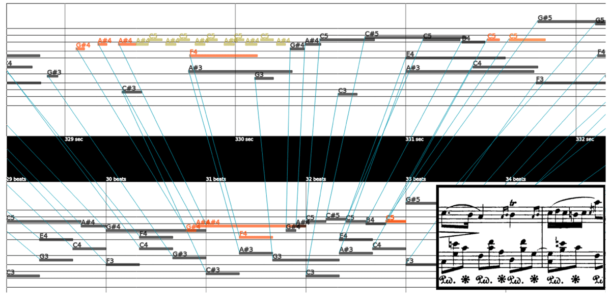
Figure 6
Parangonada visualization of an aligned excerpt of Chopin’s Nocturne Op. 32 No. 2, measures 8–9. The top piano roll represents the performance; the bottom piano roll the score. Lines connect notes aligned by automatic note alignment models. The score is added for clarity and is not part of the interface. Parangonada is not aware of pitch spelling; all black notes are displayed as ♯ even though the piece is in A♭ major.
Figure 6 shows a note-aligned excerpt from Chopin’s Nocturne Op. 32 No. 2. The top piano roll is the performance, and the bottom the score. Note alignments are represented by lines connecting notes of the performance with corresponding notes in the score. The excerpt is taken from measures 8–9, and the corresponding section of the score is added at the bottom right (taken from https://imslp.org). This excerpt showcases a number of common difficulties encountered during note alignment creation, namely three different types of ornaments—two appoggiature, an acciaccatura, and a trill—and a five-over-three cross-rhythm.
Parangonada is able to represent two alignments at the same time, e.g., for comparison of a predicted note alignment with a ground truth. By way of example, Figure 6 compares alignments produced by Nakamura’s and our DTW-based model. Blue lines represent notes matched by our DTW-based algorithm. These alignments recover the ground truth. Yellow notes are trills which are not individually marked in the score and correctly identified as insertions. A second alignment created by Nakamura’s algorithm is loaded into Parangonada. The interface allows the user to toggle between the two alignments, note alignments produced by Nakamura’s algorithm are not shown as lines. The alignment is however implicit in the color coding of notes. Orange notes indicate notes whose matching differs between the two displayed alignments. These notes are not matched by Nakamura’s algorithm but correctly matched by our DTW-based model.
5.4 Analysis of Expressive Features
Note alignment data is required for many tasks such as performance-to-score music transcription, score following, and expressive performance analysis. However, these are not the most well-known MIR tasks and it might not be clear what the benefit of note alignments is. In this section, we provide some exemplary analyses that cannot be done without reliable note alignments.
Note-aligned data can be used to compute detailed descriptions of expressive characteristics of individual notes or chords. Figure 7 shows histograms of tempo and articulation features for four composers. Local tempo as presented here is computed at each individual score onset. When multiple notes are played at the same onset, an average onset time is used for tempo computation. This results in a single tempo curve for each performance that is much more fine-grained than beat-wise tempo values. The second expressive feature presented is computed as the base two logarithm of the ratio of played duration (not taking pedalling into account) over notated duration. Interestingly, there seem to be clear non-zero modes of articulation indicating the presence of natural but composer-specific levels of “staccatoness” and “legatoness”.
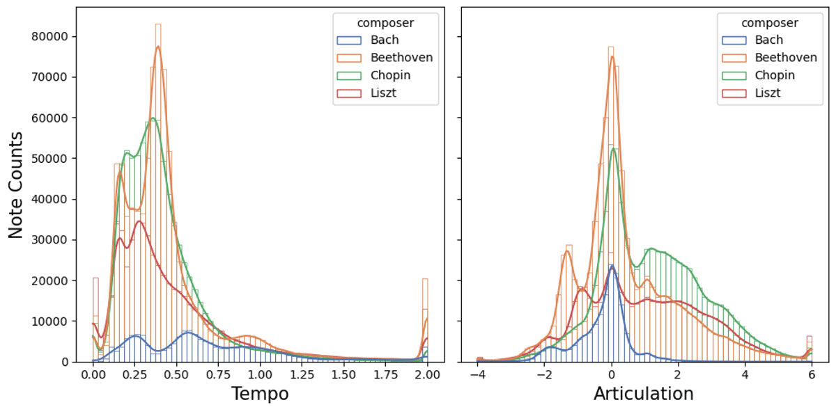
Figure 7
A histogram of the number of notes performed by composer and the performance statistics of those notes. Pieces from four composers were gathered: Chopin, Bach, Beethoven and Liszt. The left histogram plot shows onset-wise tempo in seconds per beat. The right plot shows a histogram of articulation expressed as a note-wise dimensionless logarithm of played duration divided by notated duration.
Figure 8 shows the distribution of chord spreads for the same four composers. Chord spread is based on the previous definition of a single tempo per unique score onset. If multiple notes of the same score onset (such as a chord) are played, the performed notes do not coincide perfectly. Notes with the same score onset may include notes from different staves and arpeggios. In this situation, we define chord spread as the absolute difference between the first and last performed onset of the notes in a chord. A small amount of chord spread is unavoidable due to motor noise, but it is also an important element of musical expression, e.g., performers tend to emphasize a melody in a chord, with effects on dynamics and melody lead (Goebl, 2001). Our distributional analysis reveals that chord spread shows a marked increase over time (Bach 1685–1750, Beethoven 1770–1827, Chopin 1810–1849, Liszt 1811–1886). We hypothesize that present day performers use this expressive device to communicate styles of common practice period solo piano music: from fairly restrained and precise Baroque playing to expressly free-flowing Romantic playing.
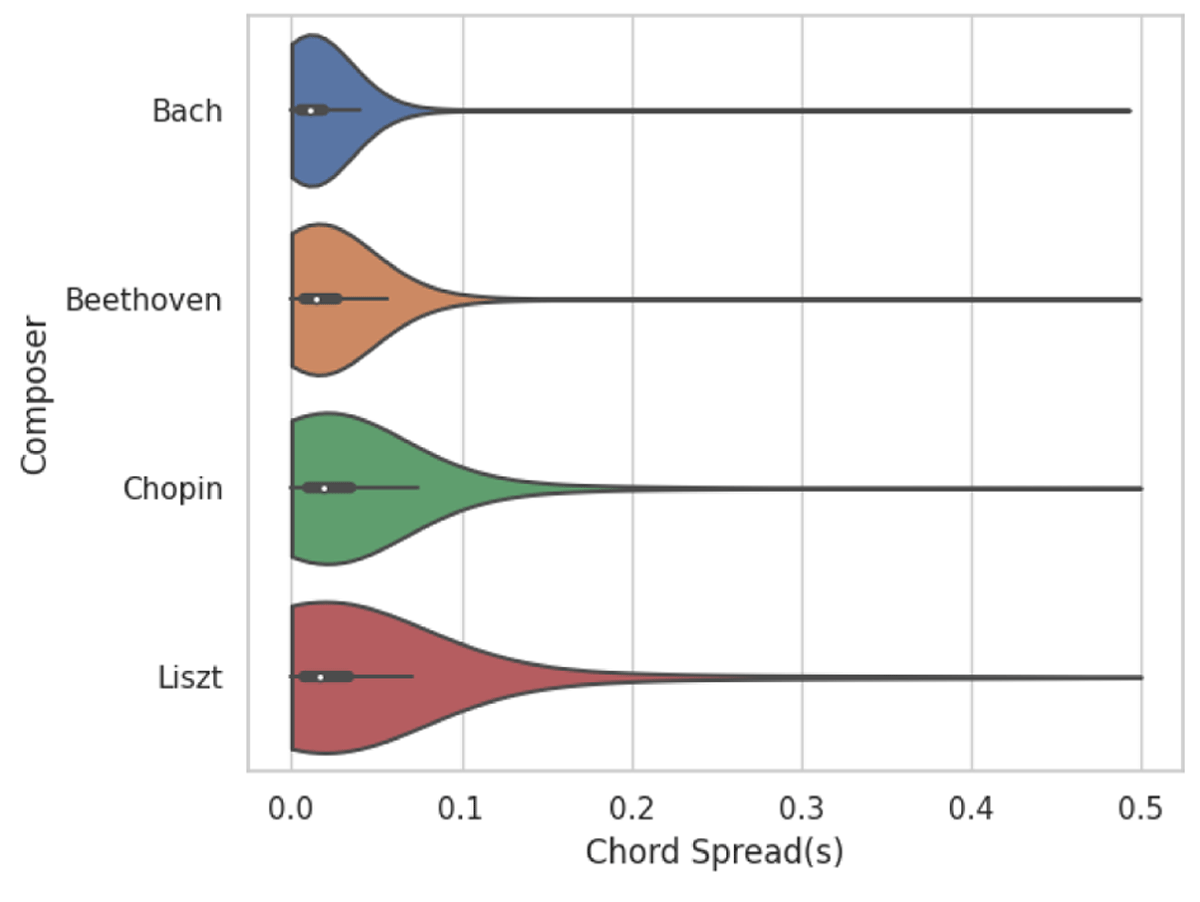
Figure 8
Chord spread distribution in seconds for four composers. Chord spread is defined for each chord as the maximal time interval between performance note onsets belonging to the chord. The white dot shows the median, the thick horizontal line the quartiles, and the thin horizontal line the 5- and 95-percentiles.
Figure 9 shows a similar analysis but much more specific. It is based on four performances of a six measure excerpt from Scriabin’s Sonata No.5, Op. 53. Violin plots represent distributions of note dynamics, local timing, and articulation for each performer (the latter two of which are impossible without a note alignment). Local timing is related to the previous definition of chord spread and refers to deviation (positive or negative) from the average performed onset of all score-coincident notes. While performer-wise distributions of expressive features of a whole piece are largely piece dependent, such local analyses can give rise to striking differences. In particular, the first and last performer play much more legato than the others, while the first performer also plays with markedly higher dynamics and looser timing.
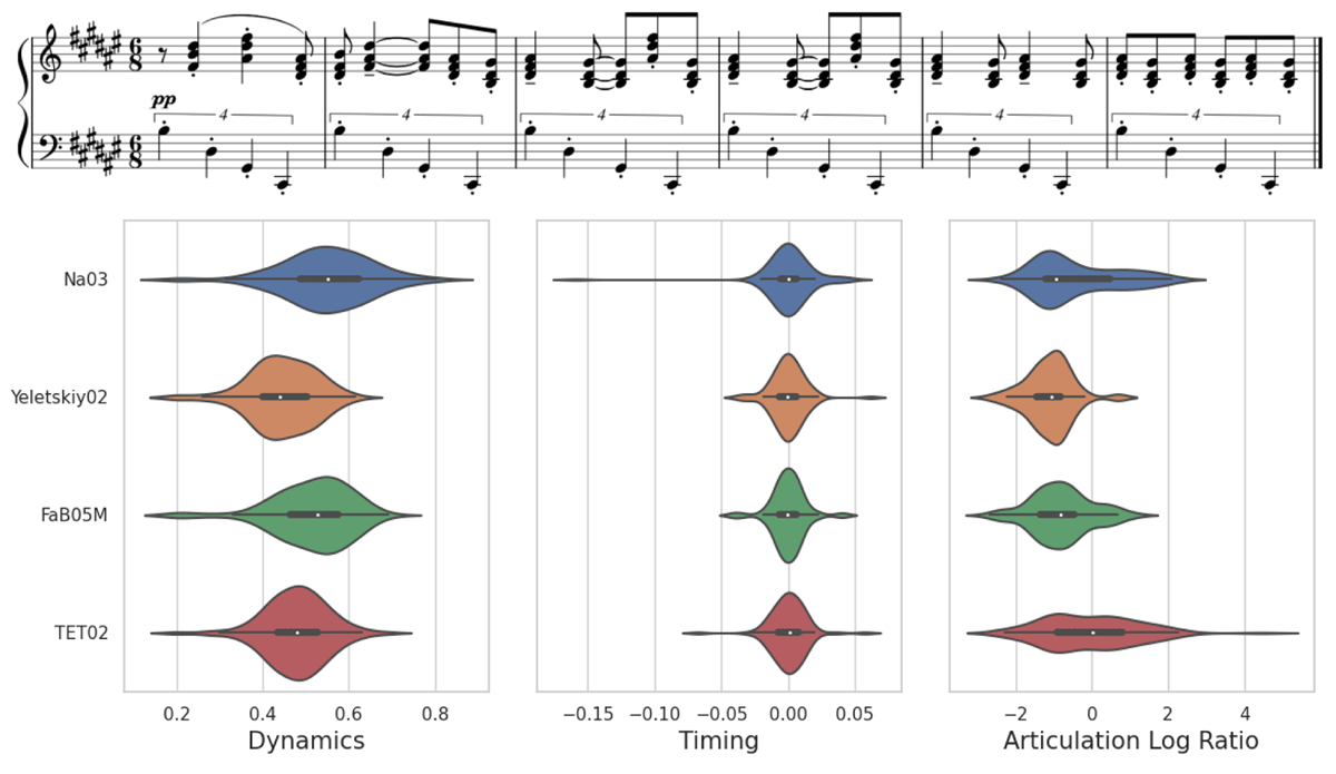
Figure 9
Performance statistics for four performers on the Scriabin Sonata No. 5, measures 47-52. Left: dynamics (MIDI velocity, normalized to (0,1)); middle: timing (how much onsets of chord notes deviate from their mean, in seconds); right: articulation (how staccato or legato the notes are played; see also Figure 7). The horizontal gray lines indicate quantiles; see also Figure 8.
6 Conclusions
In this paper, we presented four contributions: (1) a carefully note-aligned dataset (n)ASAP, produced from (2) a flexible segment-constrained alignment model, which is derived from (3) an automatic hierarchical note alignment model, and manually checked using (4) a web-based alignment correction tool.
We create new, high-quality, note alignments between the MIDI performances and the corresponding scores of the ASAP dataset. Along with this paper we publish the generated note alignments, which results in (n)ASAP, the only reliable and openly accessible resource of its size for MIR tasks that require fine-grained score information.
We present a simple and computationally inexpensive automatic note alignment model based on a hierarchical time warping step and a combinatorial symbolic note processor. This model performs on par with the current state-of-the-art models.
We adapt our model to leverage anchor points (which can be produced relatively easily, e.g., by tapping). We show that this change consistently and significantly improves the alignment performance, in particular for complex pieces that contain musical embellishments and performance errors. We also study how the results are affected by tapping noise and show that our models are robust with respect to deviations that fall in the typical human beat annotation range.
Besides our reusable models, we publish a graphical tool that facilitates the visualization of note alignment errors and their correction.
Many problems of fully automatic and segment-constrained alignment remain open. Future work includes how to handle the performed ornaments instead of simply classifying them as insertions (following previous work, e.g., Gingras and McAdams, 2011) and how to automatically detect the pieces which require anchor points, e.g., by taking cues from error identification in the related beat tracking task (Grosche et al., 2010). Furthermore, automatic error identification and correction of note alignments is an open problem.
7 Reproducibility
We publish our data, models, and tools:
(n)ASAP Dataset: https://github.com/CPJKU/asap-dataset
Alignment models: https://github.com/sildater/parangonar
Parangonada Alignment Tool: https://sildater.github.io/parangonada/.
Notes
Funding Information
This work is supported by the European Research Council (ERC) under the EU’s Horizon 2020 research & innovation programme, grant agreement No. 101019375 (“Whither Music?”), and the Federal State of Upper Austria (LIT AI Lab).
Competing Interests
The authors have no competing interests to declare.