
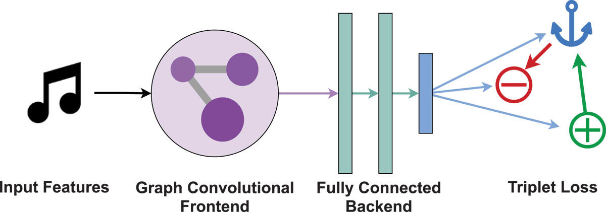
Figure 1
Overview of the graph neural network we use in this paper. First, the input features xv are passed through a front-end of graph convolution layers (see Section 3.2.2 for details); then, the output of the front-end is passed through a traditional deep neural network back-end to compute the final embeddings yv of artist nodes. Based on these embeddings, we use the triplet loss to train the network to project similar artists (positive, green) closer to the anchor, and dissimilar ones (negative, red) further away.
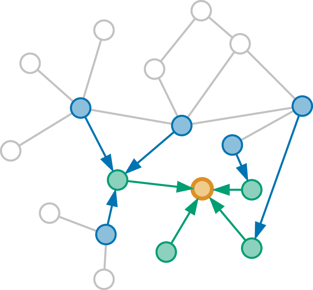
Figure 2
Tracing the graph to find the necessary input nodes for embedding the target node (orange). Each graph convolution layer requires tracing one step in the graph. Here, we show the trace for a stack of two such layers. To compute the embedding of the target node in the last layer, we need the representations from the previous layer of itself and its neighbors (green). In turn, to compute these representations, we need to expand the neighborhood by one additional step in the preceding GC layer (blue). Thus, the features of all colored nodes must be fed to the first graph convolution layer.
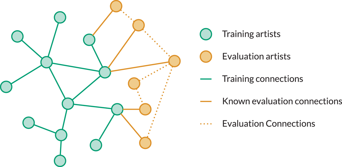
Figure 3
Artist nodes and their connections used for training (green) and evaluation (orange). During training, only green nodes and connections are used. When evaluating, we extend the graph with the orange nodes, but only add connections between validation and training artists. Connections among evaluation artists (dotted orange) remain hidden. We then compute the embeddings of all evaluation artists, and evaluate based on the hidden evaluation connections.
Table 1
NDCG@200 for the baseline (DNN) and the proposed model with 3 graph convolution layers (GNN), using features or random vectors as input. The GNN with real features as input gives the best results. Most strikingly, the GNN with random features—using only the known graph topology—out-performs the baseline DNN with informative features.
| DATASET | FEATURES | DNN | GNN |
|---|---|---|---|
| OLGA | Random | 0.02 | 0.45 |
| AcousticBrainz | 0.24 | 0.55 | |
| Proprietary | Random | 0.00 | 0.52 |
| Musicological | 0.44 | 0.57 |
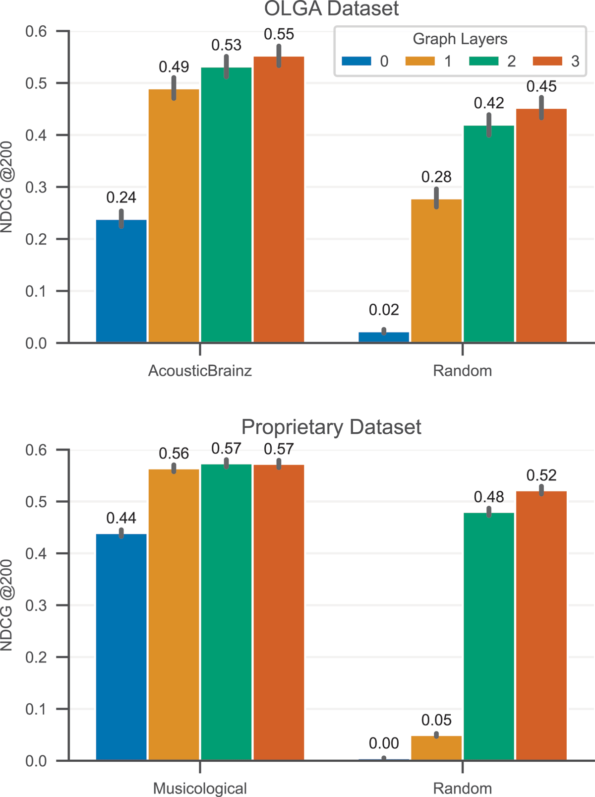
Figure 4
Results on the OLGA (top) and the proprietary (bottom) dataset with different numbers of graph convolution layers, using either the given features (left) or random vectors as features (right). Error bars indicate 95% confidence intervals computed using bootstrapping.
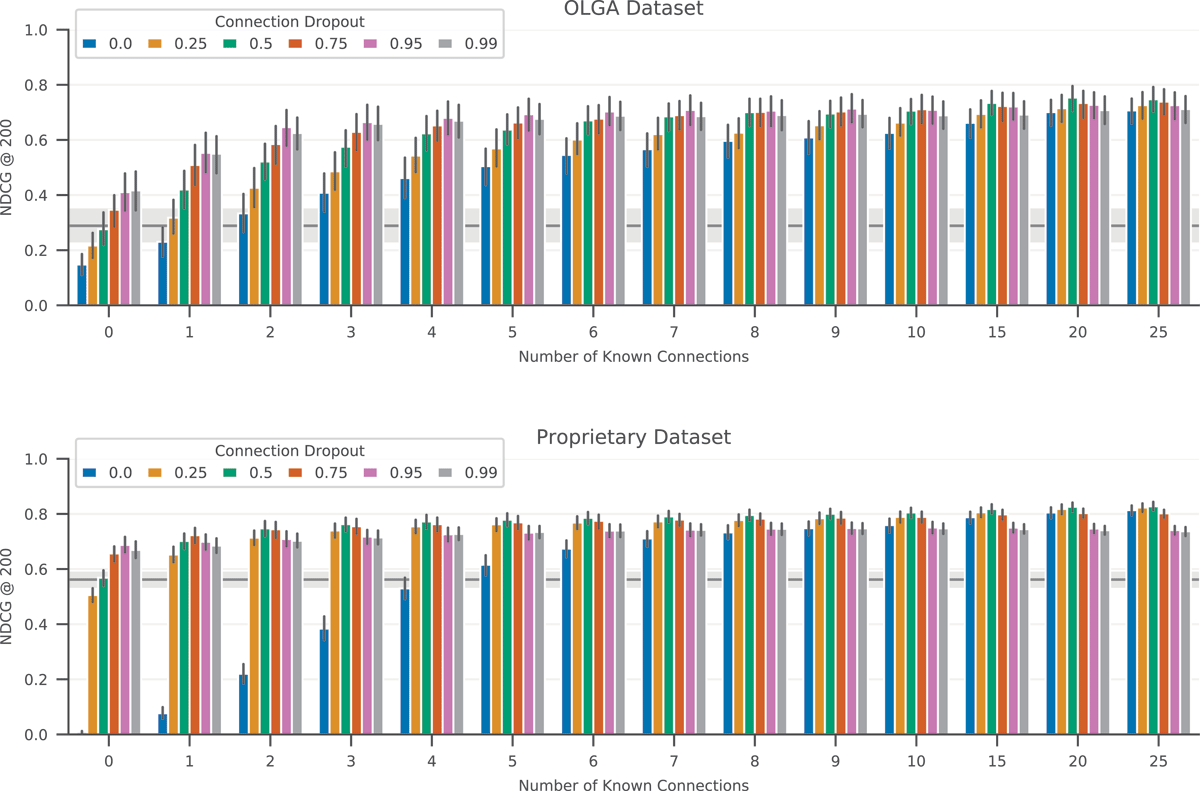
Figure 5
Evaluation of the long-tail performance of a 3-GC-layer model on the OLGA dataset (top) and the proprietary dataset (bottom). The different bars represent models trained with different probabilities of connection dropout. The gray line in the background represents the baseline model with no graph convolution layers, with the shaded area indicating the 95% confidence interval. We see that for the standard model (blue, no connection dropout), performance degrades with fewer connections. Introducing connection dropout significantly reduces this effect.

Figure 6
Cosine distance between embeddings computed using reduced connectivity and the “true” embedding (computed using all 25 known connections). Without connection dropout, the GNNs learn to rely too much on the graph connectivity to compute the artist embedding: the distance between an embedding computed using fewer connections and the “true” embedding grows quickly. With connection dropout, we can strongly curb this effect.