
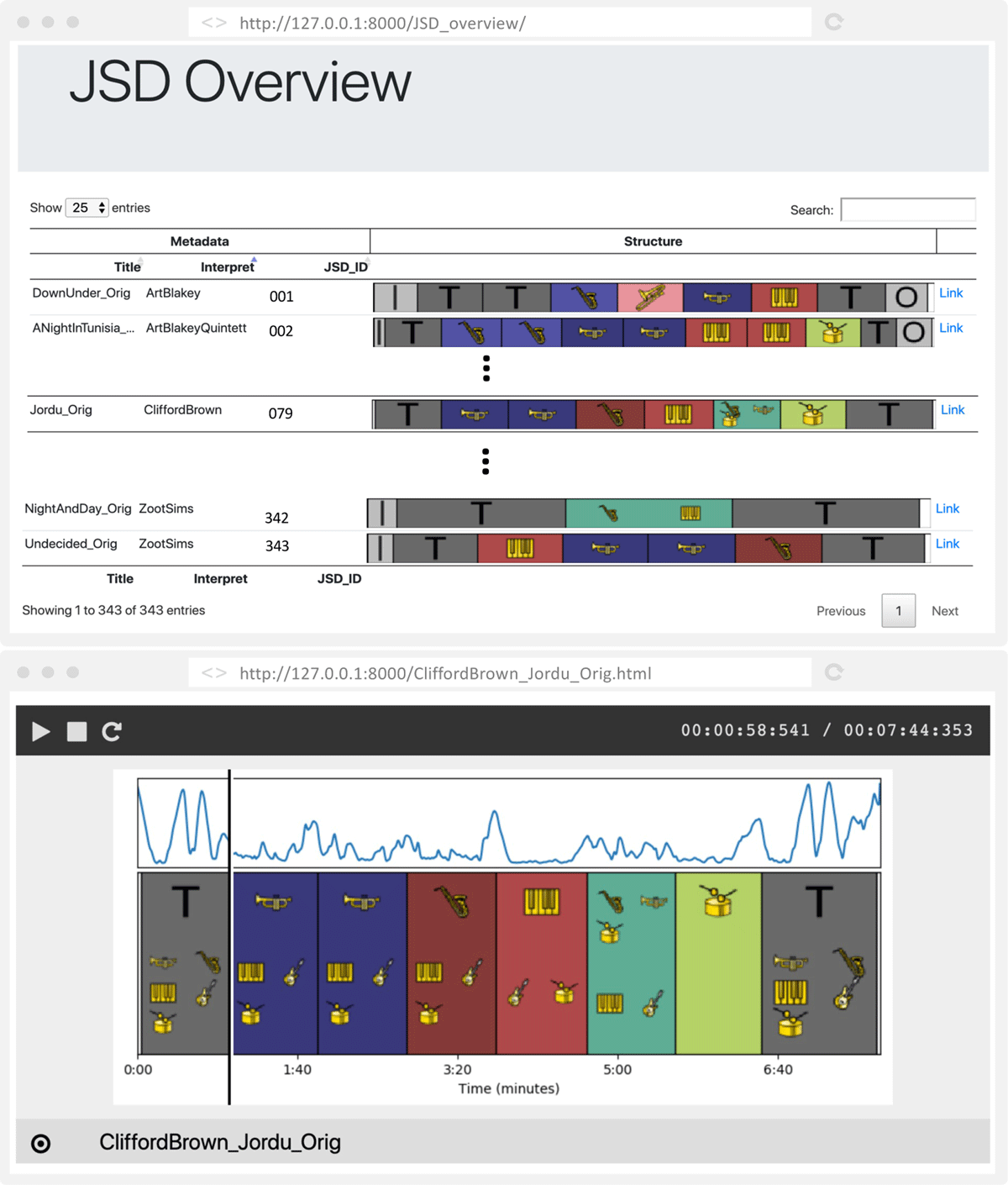
Figure 1
(a) Above: overview of the Jazz Structure dataset (JSD). (b) Below: running example “Jordu” by Clifford Brown. The figure shows a novelty function and structure annotations within a web-based interface (T = theme; the pictograms indicate the current soloist and the accompaniment).
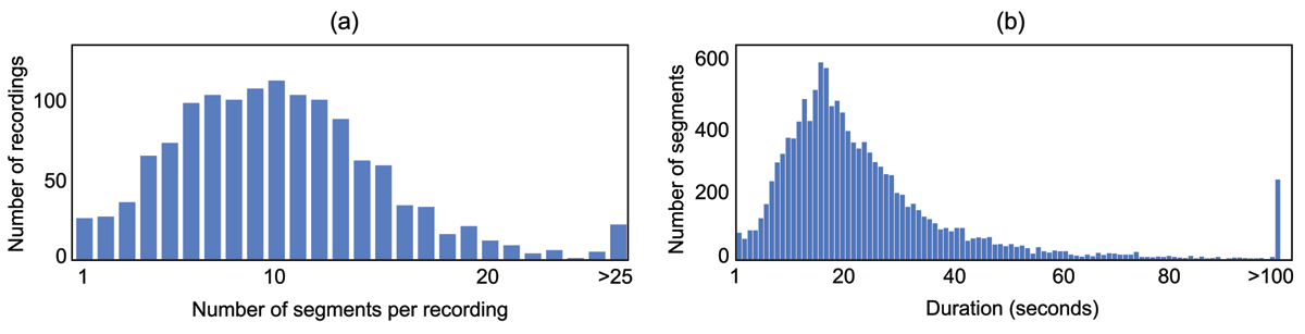
Figure 2
Statistics for the large-scale annotations of the SALAMI database. (a) Distribution of the number of segments per recording. The total number of segments is 12634. In average, each recording consists of 10.37 segments. (b) Distribution of segment durations (seconds). In average, a segment has a duration of 25.21 seconds.
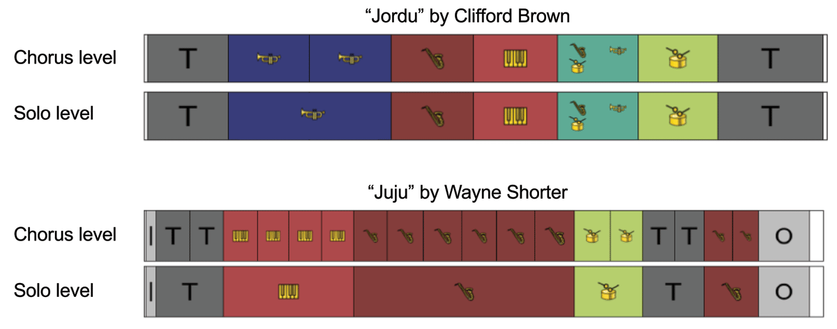
Figure 3
Examples of structure annotations on the chorus and solo level.
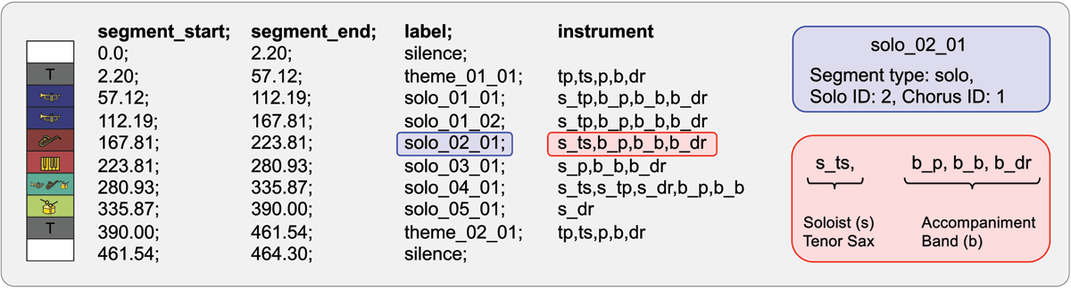
Figure 4
Raw annotation format for “Jordu” as contained in the JSD. Each row of the CSV file corresponds to a segment. The columns indicate the start time, the end time, the label, and the instrumentation of each segment.
Table 1
Overview of annotated (chorus-level) segments for the 340 recordings. From the segments, we derive 4365 segment boundaries (these include the 4025 start positions of each segment plus the 340 end positions of the last segments) from which 3005 are musical and 1360 non-musical.
| Type | # Segments | Total duration (min) |
|---|---|---|
| Intro | 229 | 59.76 |
| Theme | 813 | 546.74 |
| Solo | 2223 | 1325.31 |
| Outro | 80 | 35.15 |
| Silence | 680 | 36.93 |
| Σ 4025 | 2003.89 |
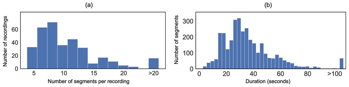
Figure 5
(a) Distribution of number of (chorus-level) segments per recording (silence segments are discarded). The total number of segments is 3345 (sum of Intro, Theme, Solo, and Outro segments, excluding silence segments). On average, a recording consists of 3345/340 ≈ 9.84 segments. (b) Distribution of segment durations (seconds) of all 3345 segments. On average, a segment has a duration of 35 seconds.
Table 2
List of instrument types occurring in JSD. The abbreviations are used as instrument identifiers. The last four columns indicate the number of solos (#Solo), the number of solo choruses (#Chorus), the number of transcribed solos (#Trans.), and the percentage of transcribed solos (%Trans.). † Note that the number of solo choruses is not identical to the number of solo segments from Table 1 (2467 vs. 2223). The former can be higher since there can be multiple soloists in a single solo section. (e.g., drums and bass).
| # | Abbr. | Instrument | #Solo | #Chorus | #Trans. | %Trans. |
|---|---|---|---|---|---|---|
| 0 | cl | Clarinet | 23 | 35 | 15 | 65.22 |
| 1 | bcl | Bass clarinet | 4 | 14 | 2 | 50 |
| 2 | ss | Soprano saxophone | 25 | 74 | 23 | 92 |
| 3 | as | Alto saxophone | 107 | 239 | 80 | 74.77 |
| 4 | ts | Tenor saxophone | 245 | 727 | 158 | 64.49 |
| 5 | bs | Baritone saxophone | 21 | 35 | 11 | 52.38 |
| 6 | tp | Trumpet | 170 | 376 | 102 | 60 |
| 7 | fln | Flugelhorn | 2 | 4 | 0 | 0 |
| 8 | cor | Cornet | 18 | 24 | 15 | 83.33 |
| 9 | tb | Trombone | 38 | 83 | 26 | 68.42 |
| 10 | p | Piano | 222 | 456 | 6 | 2.70 |
| 11 | key | Keyboard | 3 | 8 | 0 | 0 |
| 12 | vib | Vibraphone | 15 | 28 | 12 | 80 |
| 13 | voc | Vocals | 8 | 15 | 0 | 0 |
| 14 | fl | Flute | 4 | 6 | 0 | 0 |
| 15 | g | Guitar | 39 | 88 | 6 | 15.38 |
| 16 | bjo | Banjo | 1 | 1 | 0 | 0 |
| 17 | vc | Violoncello | 1 | 2 | 0 | 0 |
| 18 | b | Bass | 61 | 113 | 0 | 0 |
| 19 | dr | Drums | 65 | 131 | 0 | 0 |
| 20 | perc | Percussion | 2 | 8 | 0 | 0 |
| 1074 | 2467† | 456 | 33.75 |
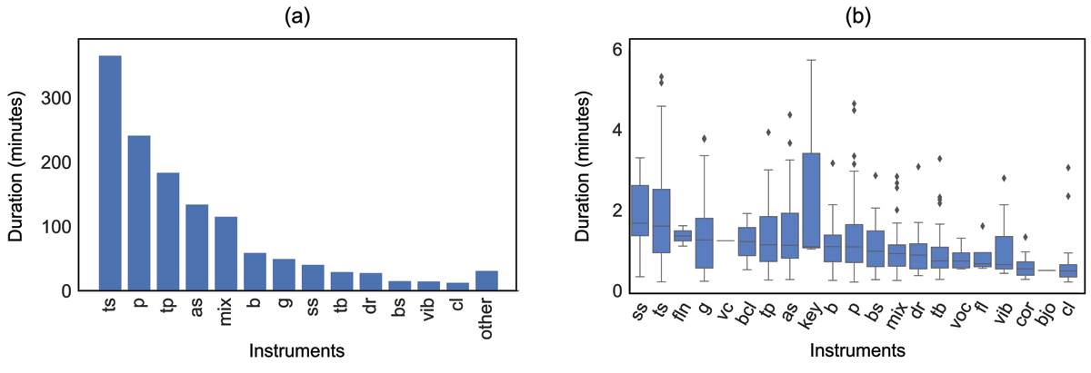
Figure 6
(a) Accumulated duration of all solos (minutes) per instrument. The total duration of all solos is 1325 minutes. (b) Statistics on durations of solo sections (seconds) broken down by instrument. The outlier “Impressions” by John Coltrane (containing a 13-minute long saxophone solo) is not shown.
Table 3
Layer structure of the CNN-based approach.
| Layer Type | Size | Output Shape |
|---|---|---|
| InputLayer | — | (116, 80, 1) |
| Batch Normalization | — | (116, 80, 1) |
| Conv2D (ReLU) | 8×6 | (109, 75, 32) |
| MaxPooling2D | 3×6 | (36, 12, 32) |
| Conv2D (ReLU) | 6×3 | (31, 10, 64) |
| Flatten | — | (19,840) |
| Dropout (50%) | — | (19,840) |
| Dense (ReLU) | — | (128) |
| Dropout (50%) | — | (128) |
| Dense (Sigmoid) | — | (1) |
Table 4
Overview of the splits for the datasets SALAMI, JSD, and SALAMI+JSD. The numbers refer to recordings (with the corresponding percentage given in brackets).
| Dataset | Training Set | Val. Set | Test Set | Σ |
|---|---|---|---|---|
| SALAMI (S) | 772 (56.8%) | 100 (7.4%) | 487 (35.8%) | 1359 |
| JSD (J) | 244 (71.7%) | 28 (8.16%) | 68 (20.1%) | 340 |
| SALAMI+JSD (S+J) | 1016 (59.9%) | 128 (7.5%) | 555 (32.7%) | 1699 |
Table 5
Evaluation results for boundary detection on the test sets of (a) SALAMI and (b) JSD. The shown precision, recall, and F-measure values are averaged over the respective test set tracks.
| (a) Evaluation results for SALAMI. | ||||||
| τ = 0.5 s | τ = 3.0 s | |||||
| P0.5 | R0.5 | F0.5 | P3 | R3 | F3 | |
| UllrichS, short | 0.422 | 0.490 | 0.422 | — | — | — |
| CNNS, short | 0.357 | 0.414 | 0.358 | 0.419 | 0.750 | 0.512 |
| CNNS, long | 0.234 | 0.223 | 0.213 | 0.563 | 0.672 | 0.580 |
| CNNJ, short | 0.231 | 0.075 | 0.100 | 0.432 | 0.420 | 0.386 |
| CNNJ, long | 0.136 | 0.049 | 0.066 | 0.494 | 0.233 | 0.287 |
| CNNS+J, short | 0.347 | 0.423 | 0.357 | 0.484 | 0.660 | 0.522 |
| CNNS+J, long | 0.242 | 0.226 | 0.221 | 0.508 | 0.729 | 0.571 |
| Footeshort | 0.227 | 0.274 | 0.223 | 0.467 | 0.610 | 0.477 |
| Footelong | 0.199 | 0.167 | 0.169 | 0.534 | 0.466 | 0.463 |
| Baseline (equal) | 0.042 | 0.041 | 0.043 | 0.237 | 0.231 | 0.244 |
| (b) Evaluation results for JSD. | ||||||
| τ = 0.5 s | τ = 3.0 s | |||||
| P0.5 | R0.5 | F0.5 | P3 | R3 | F3 | |
| CNNS, short | 0.186 | 0.230 | 0.189 | 0.297 | 0.610 | 0.382 |
| CNNS, long | 0.122 | 0.126 | 0.118 | 0.423 | 0.579 | 0.465 |
| CNNJ, short | 0.303 | 0.125 | 0.165 | 0.428 | 0.556 | 0.452 |
| CNNJ, long | 0.193 | 0.117 | 0.139 | 0.615 | 0.439 | 0.482 |
| CNNS+J, short | 0.242 | 0.269 | 0.232 | 0.409 | 0.531 | 0.428 |
| CNNS+J, long | 0.199 | 0.169 | 0.166 | 0.401 | 0.682 | 0.485 |
| Footeshort | 0.186 | 0.247 | 0.192 | 0.436 | 0.601 | 0.454 |
| Footelong | 0.216 | 0.185 | 0.184 | 0.548 | 0.505 | 0.488 |
| Baseline (equal) | 0.051 | 0.051 | 0.051 | 0.225 | 0.225 | 0.225 |
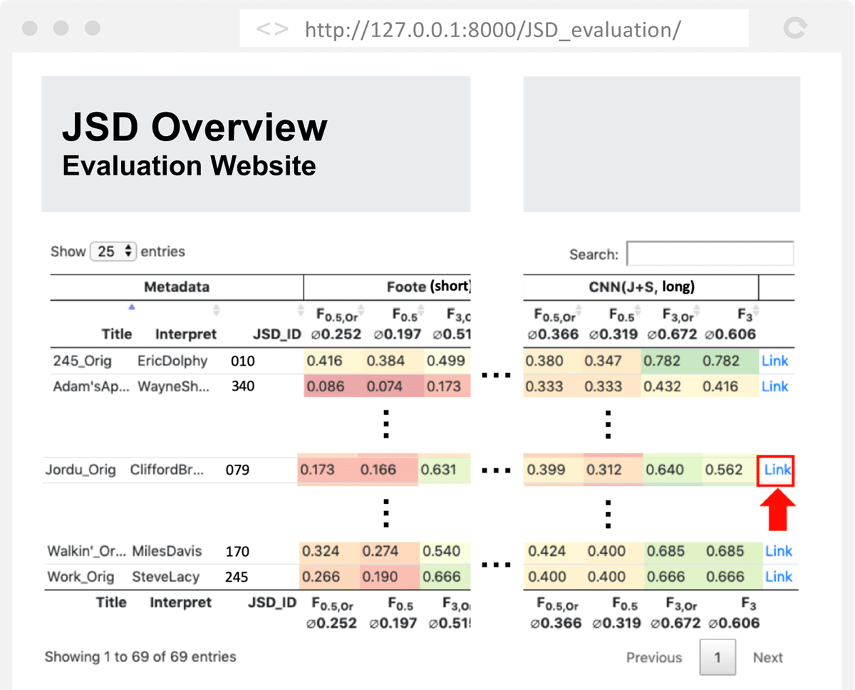
Figure 7
Overview of the evaluation results for all recordings contained in the JSD’s test set. The link (red arrow) leads to the details page as depicted in Figure 8.
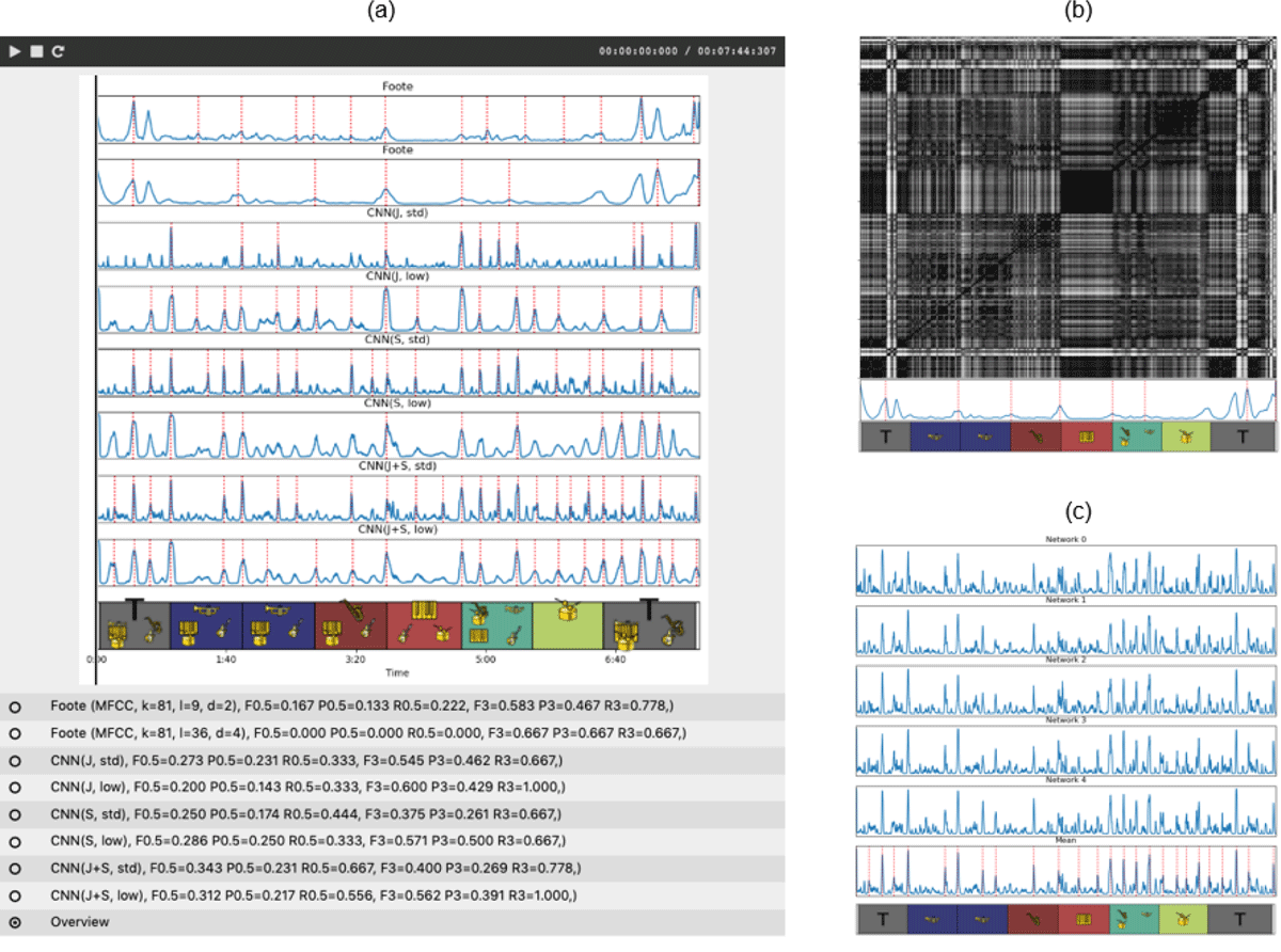
Figure 8
(a) Evaluation web page showing the output of all methods for the running example “Jordu” by Clifford Brown. (b) Evaluation results of Foote’s method with the input SSM based on MFCCs. (c) Evaluation results of a CNN consisting of the novelty curve of five networks and the bagged novelty curve.