
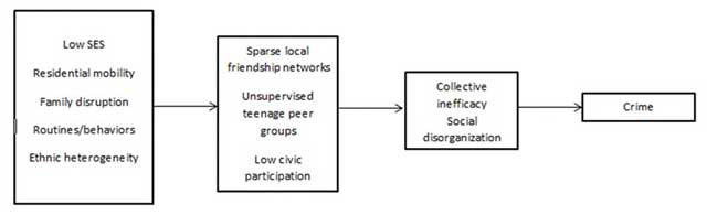
Figure 1
Social disorganization theory: structures and processes. Source: Adapted from Sampson and Groves (1989) and Sampson (2011).
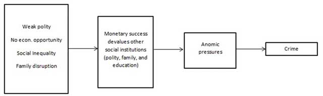
Figure 2
Institutional anomie theory: institutions and processes. Source: Adapted from Messner and Rosenfeld (1997) and Rosenfeld and Messner (2010).
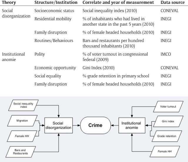
Figure 3
The correlates and data sources of social disorganization and institutional anonmie theory. Source: authors.
Table 1
Descriptive statistics for variables included in the analysis.
| Mean | S. D. | |
|---|---|---|
| Rates for all crimes (per 100,000) | 1471.6 | 1033.5 |
| Social lag index | −1.146 | 0.403 |
| Migration % | 5.4% | 5.1% |
| Bars/restaurants (per 100,000) | 10.6 | 17.8 |
| Female HH % | 20.3% | 4.7% |
| Voter turnout % | 54.2% | 10.6% |
| Gini index | 0.402 | 0.034 |
| Grade retention % (primary school) | 96.9% | 1.3% |
[i] Note: All variables transformed to Z values prior to inferential analyses (n = 76).
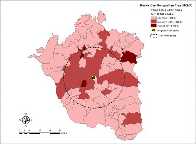
Map 1
Spatial distribution of crime rates, 2010. Source: authors based on 2010 crime data (INEGI).
Map 2
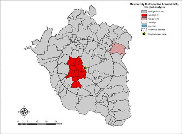
Crime hotspots, 2010. Source: Author calculations based on 2010 crime data (INEGI).
Table 2
Crime hot spots, 2010.
| Type of hotspot | State | Municipality | Crime rate for all crimes (2010)** |
|---|---|---|---|
| High-High | Distrito Federal | Cuauhtemoc | 5,418.1 |
| High-Low | Estado de Mexico | Otumba | 4,048.8 |
| High-High | Distrito Federal | Benito Juarez | 3,561.7 |
| High-High | Distrito Federal | Miguel Hidalgo | 3,522.8 |
| High-High | Distrito Federal | Venustiano Carranza | 2,979.3 |
| High-High | Estado de Mexico | Tlalnepantla de Baz* | 2,661.7 |
| High-High | Distrito Federal | Azcapotzalco | 2,267.6 |
| High-High | Distrito Federal | Coyoacan | 2,152.9 |
| High-High | Distrito Federal | Iztacalco | 2,107.8 |
| High-High | Distrito Federal | Gustavo A. Madero | 1,990.6 |
[i] Source: Author calculations based on 2010 crime data (INEGI).
*This municipality is made-up of two separated geographical areas.
**Criminal investigations per hundred thousand inhabitants.
Table 3
Zero order correlations between variables included in the analysis.
| Social lag index | Migration | Bars / restaurants | Female HH | Voter turnout | Gini index | Grade retention | |
|---|---|---|---|---|---|---|---|
| Rates for all crimes | −0.618** | 0.230* | 0.382** | 0.694** | −0.554** | 0.449** | −0.065 |
| Social lag index | −0.275* | −0.182 | −0.650** | 0.634** | −0.393** | 0.164 | |
| Migration | 0.050 | −0.027 | −0.271* | 0.055 | −0.513** | ||
| Bars / restaurants | 0.429** | −0.078 | 0.307** | 0.213 | |||
| Female HH | −0.666** | 0.487** | 0.199 | ||||
| Voter turnout | −0.383** | 0.112 | |||||
| Gini index | 0.313** |
Table 4
OLS regression analysis of crime rates on measures of social disorganization and institutional anomie theories w/interactions.
| Model 1 Social Disorganization | Model 2 Institutional Anomie | Model 3 Full model | |
|---|---|---|---|
| Social lag index | −0.217* | – | −0.095 |
| Migration % | 0.178** | – | 0.111 |
| Bars/restaurants per capita | 0.115 | – | 0.022 |
| Female HH % | 0.508*** | 0.500*** | 0.491*** |
| Voter turnout % | – | −0.080 | −0.025 |
| Gini index | – | 0.356*** | 0.296*** |
| Grade retention % | – | −0.261*** | −0.163 |
| Gini*Female HH% | – | 0.260*** | 0.225** |
| Gini*Voter turnout % | – | 0.164** | 0.188** |
| Gini*Grade retention % | – | −0.239*** | −0.223*** |
| intercept | 0.001 | 0.010 | 0.031 |
| R2 adjusted | 0.542 | 0.564 | 0.558 |
[i] Note: Significance of the coefficients based on robust standard errors.
*p < 0.1, **p < 0.05, ***p < 0.01.
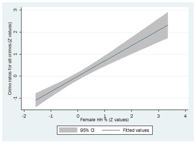
Figure 4
Female-headed households as the strongest predictor of crime rates for all crimes Source: Author calculations.
Table 5
GWR regression analysis of crime rates on measures of social disorganization and institutional anomie theories w/o interactions (mean values).
| Model 1 Social Disorganization | Model 2 Institutional Anomie | Model 3 Full model | |
|---|---|---|---|
| Social lag index | −0.262 | – | −0.113 |
| Migration % | 0.175 | – | 0.106 |
| Bars/restaurants per capita | 0.133 | – | 0.037 |
| Female HH % | 0.467 | 0.494 | 0.461 |
| Voter turnout % | – | −0.079 | −0.040 |
| Gini index | – | 0.352 | 0.287 |
| Grade retention % | – | −0.258 | −0.167 |
| Gini*Female HH% | – | 0.257 | 0.225 |
| Gini*Voter turnout % | – | 0.162 | 0.180 |
| Gini*Grade retention % | – | −0.236 | −0.222 |
| Intercept | −0.002 | −0.011 | 0.026 |
| R2 adjusted | 0.571 | 0.564 | 0.568 |
| Bandwidth size | 51 | 76 | 62 |
[i] Note: Mean values of local standardized beta coefficients reported (n = 76).
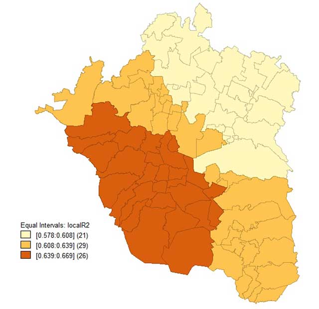
Map 3
Social disorganization theory model: GWR local coefficients of determination, 2010. Source: Author calculations.
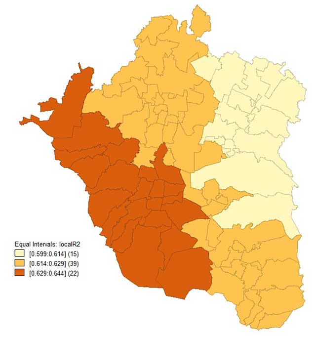
Map 4
Institutional anomie theory model: GWR local coefficients of determination, 2010. Source: Author calculations.
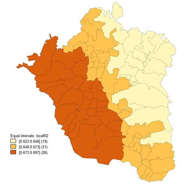
Map 5
Social disorganization and Institutional theory model: GWR local coefficients of determination, 2010.