
Introduction
Salt marsh foraminifera have been utilized by many authors as an excellent biological proxy for palaeoenvironmental studies, including precise Holocene sea-level indicators (e.g., Scott & Medioli 1978; Gehrels 1994; Scott, Medioli & Schafer 2004). The understanding of former sea-levels based on the interpretation of foraminiferal assemblages requires that their relationship to tidal elevation is known (Scott & Medioli 1978; Horton, Edwards & Llyod 1999; Horton & Edwards 2006), and it differs among sites and regions (Kemp et al. 2013). Recently, a transfer function has been developed based on the statistically significant relationship between foraminiferal assemblages (modern data sets) and elevation with respect to the tidal frame (e.g., Gehrels 2000; Horton, Edwards & Llyod 1999; Horton & Edwards 2006; Leorri, Horton & Cearreta 2008; Kemp et al. 2013), which can be used to infer the former heights of fossil salt marsh deposits (Berkeley et al. 2007). An ideal modern foraminiferal assemblage to be used in sea-level studies must be shown to correspond to environmental gradients, to be autochthonous and must remain compositionally similar with their subsurface (dead) assemblages throughout the core (Horton & Edwards 2006; Berkeley et al. 2007; Edwards & Wright 2015).
Dead subsurface assemblages that accurately reflect the dead surface assemblage indicate low taphonomic processes (Horton & Edwards 2006) and suitability to be used in palaeoenvironmental studies. However, other studies reported that occurrences of infaunal foraminifera could influence the composition of dead assemblages in subsurface sediments and lead to erroneous conclusions regarding their original composition (e.g., Goldstein & Harben 1993; Goldstein, Watkins & Kuhn 1995; Saffert & Thomas 1998; Culver & Horton 2005; Horton & Edwards 2006; Culver et al. 2013), which resulted in biased interpretation of palaeo sea-level and palaeoenvironmental studies. In this context, subsurface dead assemblages should therefore be evaluated to optimize the accuracy of palaeoenvironmental interpretations (Goldstein & Harben 1993).
Goldstein et al (1995) characterized the mode of living of salt marsh foraminifera into three; 1) predominantly epifaunal (allogromiinans, most monothalamous agglutinated taxa, and miliolids); 2) shallow to intermediate infaunal (0–5 cm or 9–11 cm) (e.g., Ammonia beccarii, Miliammina fusca, Pseudothurammina limnetis, Ammotium salsum, Ammobaculites dilatatus, Reophax nana, Textularia palustris, Siphotrochammina lobata, Trochammina inflata, and T. macrescens); and 3) deep infaunal (deeper than 10 cm) (e.g., Arenoparrella mexicana, Haplophragmoides wilberti). However, the distinction between epifaunal and shallow infaunal may be negligible if the sediment is soft (Murray, 2003). In our study sites, the mangrove sediments are muddy and soft and therefore, the term infaunal (shallow and deep) is used to represent our foraminiferal mode of living.
Abundance and distribution patterns of infaunal foraminifera vary considerably from site to site, due to local environmental conditions and bioturbation (Culver & Horton 2005). In temperate regions, infaunal foraminifera have been reported at a depth of 60 cm in Delaware salt marshes (Hippensteel et al. 2000) and at a depth of 50 cm in New England salt marshes (Saffert & Thomas 1998). At a site that was located around ~150 km north from this present study, Culver et al. (2013) reported the first infaunal foraminiferal occurrences in Malaysia and the deepest in this region; 78–80 cm in Setiu estuary and lagoon. In comparison with salt marshes in temperate regions, mangrove foraminifera from tropical environment received less attention even though intertidal zonation was proven to be established (Haslett, 2001; Horton et al. 2005). This study therefore, aimed to document the dead and living infaunal populations of foraminifera from a tropical mangrove environment and their taphonomic inferences.
Regional Setting
In the Kemaman district of Terengganu, east coast Peninsular Malaysia, mangrove swamps are highly distributed in estuaries and along tidal segments of rivers in Chukai, Kertih, Kemaman and Kemasik (Figure 1). Due to higher wave energy from the South China Sea, mangrove swamps are less extensive along the east coast than the west coast of Peninsular Malaysia (Husain & Yaakob 1995; Husain & Sulong 2001; Sulong et al. 2002). The relatively pristine mangrove swamps have been gazetted as a mangrove forest reserve by the Terengganu Forestry Department. The dominant mangrove species includes Rhizophora, Avicennia and Xylocarpus spp. (Sulong et al. 2002; Kamaruzzaman & Ong 2008; Shaari et al. 2020).
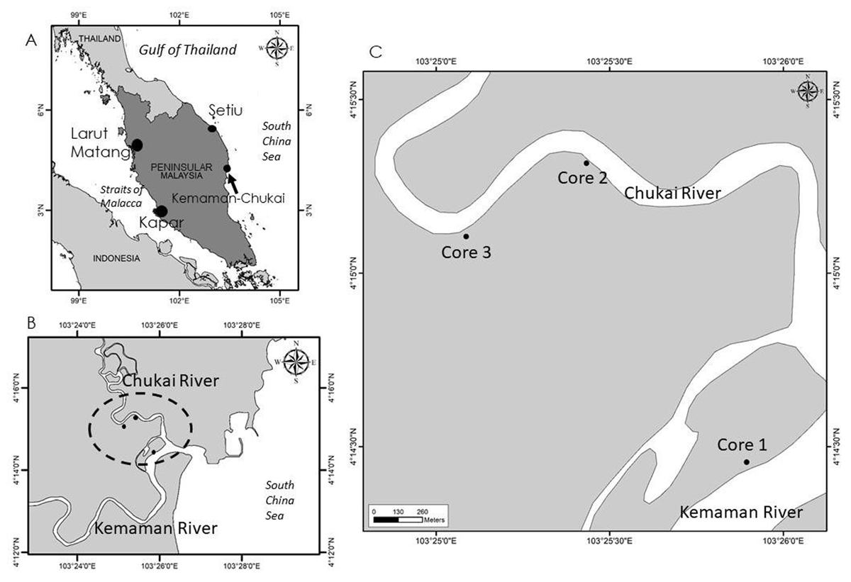
Figure 1
Location of the study area: A) showing some of the mangrove swamp areas in Peninsular Malaysia (Larut Matang and Kapar in the west coast of Peninsular, Setiu and Kemaman-Chukai in the east coast of Peninsular). Arrow indicates the location of Kemaman-Chukai; B and C) showing the location of the three sites selected in the present study; Core 1, Core 2, Core 3.
The wet equatorial climate of the study area is characterized by high temperatures and seasonally heavy rainfall, especially during the annual northeast monsoon from November to January. The mean maximum and minimum annual temperatures are 32.7°C and 24.2°C respectively, and in Peninsular Malaysia, the total rainfall recorded is between 1800 mm to 3900 mm (Malaysian Meteorological Service 2019). Tides are asymmetric but predominantly diurnal with a mean tidal range of 1.8 m. During the highest astronomical tides, tidal range can exceed 2 m. Tidal intrusion into the rivers can reach up to 20 km (Kamaruzzaman 1994). Sedimentation rates within the Kemaman-Chukai mangroves range from 0.9 to 1.1 cm year–1 (Kamaruzzaman & Ong 2008). Sediment characteristics are influenced by monsoon season, where sand content is higher during dry season and finer sediment is dominant during wet season (Ong et al. 2012).
Material and Methods
Sample Collection and Analyses
Field sampling in the Kemaman Forest Reserve was conducted in July 2009. Three sites were selected (Table 1 and Figure 1); Core 1 (seaward core) was located on the northern part of Che Wan Dagang Island near the confluence of the Kemaman and Chukai rivers (Figure 1). Core 2 (middle core) and Core 3 (landward core) were located about 2 km and 4 km, respectively, up the Chukai River (Figure 1).
Table 1
Location, depth interval, salinity, elevation level relative to mean sea-level (MSL), sediment types, total organic carbon, dominant vegetation, number of dead and live foraminifera and diversity indices of 15 sediment subsamples taken from three cores in the Kemaman-Chukai mangrove swamp.
| SUBSAMPLE DEPTH INTERVAL (CM) | SALINITY (PPT) | ELEVATION MSL (M) | SEDIMENT CLASSIFICATION | TOC (%) | DOMINANT VEGETATION | NO. DEAD SPECIMENS | DOWN-CORE % OF DEAD SPECIMENS | NO. LIVE SPECIMENS | DOWN-CORE % OF LIVE SPECIMENS | S (DEAD/LIVE) | α (DEAD/LIVE) | H’ (DEAD/LIVE) | J’ (DEAD/LIVE) | |
|---|---|---|---|---|---|---|---|---|---|---|---|---|---|---|
| Core 1 (04°14’39’’N, 103°25’53’’E) | ||||||||||||||
| C1S1 | 0–1 | 32 | 1.7 | Sand | 5.4 | Rhizophora apiculata | 1 | 2.9 | 0 | 0 | 1/0 | 0/0 | 0/0 | 0/0 |
| C1S2 | 10–11 | Muddy sand | 5.7 | 16 | 45.7 | 0 | 0 | 6/0 | 3.5/0 | 1.6/0 | 0.9/0 | |||
| C1S3 | 20–21 | Muddy sand | 5.1 | 7 | 20.0 | 0 | 0 | 2/0 | 0.9/0 | 0.6/0 | 0.9/0 | |||
| C1S4 | 30–31 | Sandy mud | 5.9 | 9 | 25.7 | 0 | 0 | 5/0 | 4.6/0 | 1.5/0 | 0.9/0 | |||
| C1S5 | 40–41 | Sandy mud | 4.9 | 2 | 5.7 | 0 | 0 | 1/0 | 0/0 | 0/0 | 0/0 | |||
| Total: 35 | Total: 100 | Total: 0 | Total: 0 | |||||||||||
| Core 2 (04°15’19’”N, 103°25’26”’E) | ||||||||||||||
| C2S1 | 0–1 | 28 | 2 | Sandy mud | 5.6 | Rhizophora apiculata | 68 | 24.6 | 3 | 50 | 10/1 | 3.2/0 | 1.7/0 | 0.8/0 |
| C2S2 | 10–11 | Sandy mud | 5.9 | 75 | 27.2 | 2 | 33.3 | 12/1 | 4/0 | 1.8/0 | 0.7/0 | |||
| C2S3 | 20–21 | Mud | 5.4 | 8 | 2.9 | 0 | 0 | 6/0 | 10.9/0 | 1.7/0 | 1.0/0 | |||
| C2S4 | 30–31 | Muddy sand | 5.4 | 81 | 29.3 | 1 | 16.7 | 9/1 | 2.6/0 | 1.4/0 | 0.6/0 | |||
| C2S5 | 40–41 | Sandy mud | 5.1 | 44 | 15.9 | 0 | 0 | 9/0 | 3.4/0 | 1.8/0 | 0.8/0 | |||
| Total: 276 | Total: 100 | Total: 6 | Total: 100 | |||||||||||
| Core 3 (04°15’6”’N, 103°25’2”’E) | ||||||||||||||
| C3S1 | 0–1 | 28 | 1.2 | Sandy mud | 5.9 | Xylocarpus granatum, Nypa fruticans | 194 | 25.0 | 18 | 47.4 | 13/2 | 3.1/0.6 | 1.5/0.5 | 0.6/0.7 |
| C3S2 | 10–11 | Sandy mud | 5.7 | 147 | 18.9 | 11 | 28.9 | 10/2 | 2.4/0.7 | 1.2/0.7 | 0.5/1.0 | |||
| C3S3 | 20–21 | Mud | 5.7 | 150 | 19.3 | 0 | 0 | 12/0 | 3.1/0 | 1.4/0 | 0.5/0 | |||
| C3S4 | 30–31 | Muddy sand | 5.8 | 139 | 17.9 | 5 | 13.2 | 12/0 | 3.2/1.2 | 1.6/0.7 | 0.7/1.0 | |||
| C3S5 | 40–41 | Sandy mud | 5.7 | 147 | 18.9 | 4 | 10.5 | 14/0 | 3.8/0 | 1.8/0 | 0.7/0 | |||
| Total: 777 | Total: 100 | Total: 38 | Total: 100 | |||||||||||
Cores were collected using a D-section (Russian) corer (50 cm) during low tide and from muddy substrates for easy penetration of the corer (Figure 2). Coring sites were also established far from root systems and crab mounds whenever possible. Due to the lithological homogeneity of the sediment throughout the core, the cores were sectioned at every 10 cm (e.g., 0–10 cm), and each section were divided into two parts (vertically) for foraminiferal and environmental analyses purposes. For foraminiferal analysis, 10 g of sediment were subsampled from the top 1 cm of each section, wrapped in polythene sample bags, and labelled (e.g., C1S1 = Core 1, subsample 0–1 cm).
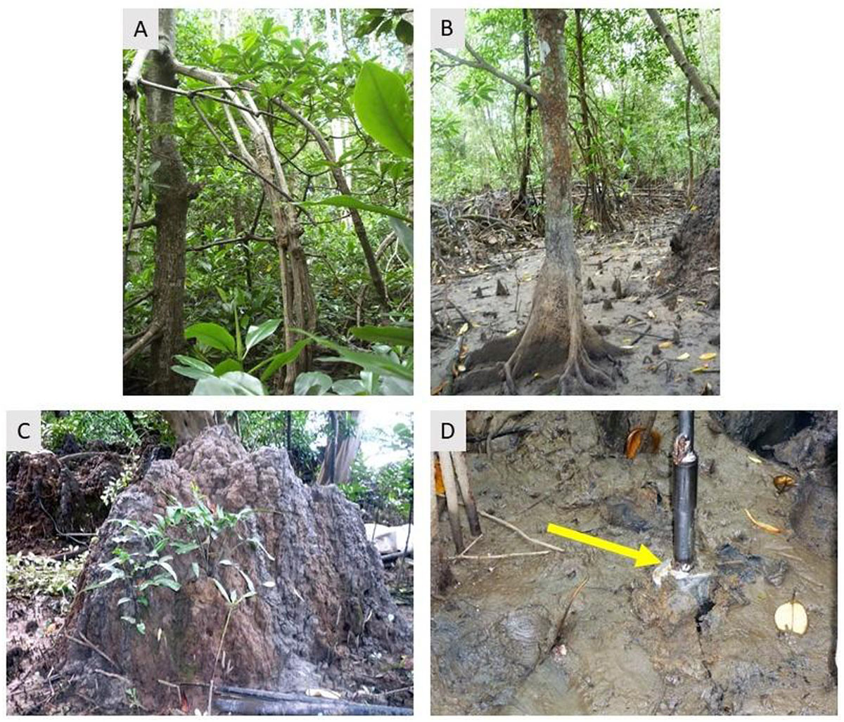
Figure 2
Root systems of Rhizophora apiculata (A) and Xylocarpus granatum (B) at the sampling sites. Subset C showing a huge (±1 m height) crab mound found at the seaward site (Core 1) of Kemaman-Chukai mangrove. Yellow arrow in subset D showing soft and muddy sediment were sampled using a D-section (Russian) corer during low tide.
To avoid bacterial oxidation and destruction of the organic wall of the foraminiferal test, all foraminiferal sediment samples were gently washed under slow-running tap water within 36 hours of collection (usually much less). Caution must be exercised, as the agglutinants are known to be very fragile and to avoid loss of foraminifera during the procedure. After washing over 600 and 63 µm sieves to remove coarse material and mud, the sample fractions retained on the small sieve were preserved in 10% formalin and 0.1% Rose Bengal (Walton 1952) mixture for preservation and staining of live foraminifera for about two to three weeks. The Rose Bengal method remains the most practical way to quantify living foraminiferal fauna (Martin 2000) and can lead to 96% correct identifications (Lutze & Altenbach 1991). Live specimens were identified by the presence of Rose Bengal stained protoplasm in their test (Wang et al. 2016). Only specimens with >50% stained test were considered as living.
Laboratory Analysis for Foraminifera
Before picking procedure started, samples were washed again in tap water to remove the formalin. Preserved foraminiferal samples were poured onto a petri dish and the foraminifera were picked in a wet medium, sorted and identified. Living and dead specimens were counted separately to provide information on living microfauna (Debenay, Guiral & Parra 2002). Due to the very low foraminiferal density, less than 300 individuals were picked in each sample. Foraminifera were identified to the species level following Loeblich & Tappan 1964; Whittaker & Hodgkinson 1979; Oki 1989; Hottinger, Halicz & Reiss 1993; and Culver et al. 2013.
Environmental Parameters
Pore water salinity data were obtained by collecting water from crab holes and small ditches at every coring site and measured using a handheld salinity refractometer. The land elevation in relation to mean sea-level (MSL) was determined using a TOPCON® (AT-G7 N, Japan) dumpy level surveying equipment. The grain size analysis was carried out through laser diffraction method (Malvern Particle Size Analyser) and then followed the Folk’s (1954) classification. However, in the case of seaward samples with a high sand fraction, the dry sieving method using British Standard sieves (63 µm) was employed. The oxidation dichromate acid technique (Holme & McIntyre 1971) was used for total organic carbon (TOC) analysis.
Data Analyses
Shannon-Wiener Information Function (H’) and Fisher’s alpha index (α) were used to measure the species diversity indices. Pielou’s evenness index (J’) was used to describe how individuals were divided among species; the greater the dominance of one species, the lower the value of evenness. Values of H’, α, and J’ were calculated using PRIMER version 6.1.12 (Clarke & Gorley 2006).
Results
The 15 sediment core subsamples collected from Kemaman-Chukai mangrove swamps contained 18 agglutinated taxa, while no presence of calcareous hyaline and calcareous porcelaneous were recorded (Table 2). The number of dead and live foraminifera recovered varied from core to core, as did their depth of occurrence.
Table 2
Foraminiferal census data for dead and live specimens in 15 sediment subsamples taken from three cores in the Kemaman-Chukai mangrove swamp. D = dead, L = live.
| CORE 1 | CORE 2 | CORE 3 | |||||||||||||
|---|---|---|---|---|---|---|---|---|---|---|---|---|---|---|---|
| Depth (cm) → | 0–1 | 10–11 | 20–21 | 30–31 | 40–41 | 0–1 | 10–11 | 20–21 | 30–31 | 40–41 | 0–1 | 10–11 | 20–21 | 30–31 | 40–41 |
| Taxa↓ | D/L | D/L | D/L | D/L | D/L | D/L | D/L | D/L | D/L | D/L | D/L | D/L | D/L | D/L | D/L |
| Acupeina triperforata | 0/0 | 0/0 | 0/0 | 0/0 | 0/0 | 0/0 | 1/0 | 0/0 | 0/0 | 0/0 | 7/0 | 2/0 | 3/0 | 7/0 | 5/0 |
| Ammoastuta salsa | 0/0 | 0/0 | 0/0 | 0/0 | 0/0 | 0/0 | 2/0 | 0/0 | 0/0 | 0/0 | 6/0 | 4/0 | 1/0 | 0/0 | 0/0 |
| Ammotium pseudocassis | 0/0 | 0/0 | 0/0 | 0/0 | 0/0 | 0/0 | 1/0 | 0/0 | 0/0 | 0/0 | 3/0 | 4/0 | 1/0 | 2/0 | 2/0 |
| Ammotium salsum | 0/0 | 0/0 | 0/0 | 0/0 | 0/0 | 0/0 | 0/0 | 0/0 | 0/0 | 0/0 | 3/0 | 0/0 | 0/0 | 0/0 | 0/0 |
| Ammotium sp. | 0/0 | 0/0 | 0/0 | 0/0 | 0/0 | 1/0 | 3/0 | 1/0 | 0/0 | 1/0 | 0/0 | 0/0 | 0/0 | 0/0 | 0/0 |
| Arenoparrella mexicana | 0/0 | 6/0 | 5/0 | 1/0 | 2/0 | 31/0 | 32/0 | 1/0 | 43/1 | 19/0 | 108/3 | 98/5 | 87/0 | 65/2 | 66/0 |
| Bruneica clypea | 0/0 | 0/0 | 0/0 | 0/0 | 0/0 | 0/0 | 1/0 | 0/0 | 1/0 | 5/0 | 0/0 | 0/0 | 1/0 | 2/0 | 5/0 |
| Caronia exilis | 0/0 | 3/0 | 0/0 | 2/0 | 0/0 | 3/0 | 3/0 | 1/0 | 1/0 | 2/0 | 3/0 | 0/0 | 1/0 | 0/0 | 3/0 |
| Entzia sp. | 0/0 | 0/0 | 0/0 | 0/0 | 0/0 | 5/0 | 13/0 | 0/0 | 0/0 | 7/0 | 3/0 | 3/0 | 9/0 | 0/0 | 2/0 |
| Haplophragmoides manilaensis | 0/0 | 0/0 | 0/0 | 0/0 | 0/0 | 7/0 | 0/0 | 0/0 | 0/0 | 0/0 | 0/0 | 0/0 | 0/0 | 1/0 | 1/0 |
| Haplophragmoides wilberti | 0/0 | 0/0 | 0/0 | 0/0 | 0/0 | 3/0 | 6/0 | 0/0 | 2/0 | 4/0 | 19/0 | 18/0 | 33/0 | 34/0 | 23/0 |
| Miliammina obliqua | 0/0 | 0/0 | 0/0 | 0/0 | 0/0 | 0/0 | 1/0 | 0/0 | 1/0 | 0/0 | 1/0 | 3/0 | 1/0 | 3/0 | 2/0 |
| Miliammina fusca | 0/0 | 1/0 | 2/0 | 0/0 | 0/0 | 9/3 | 10/2 | 1/0 | 13/0 | 2/0 | 34/15 | 11/6 | 7/0 | 11/3 | 21/4 |
| Paratrochammina sp. | 1/0 | 3/0 | 0/0 | 0/0 | 0/0 | 7/0 | 0/0 | 2/0 | 15/0 | 3/0 | 1/0 | 0/0 | 0/0 | 0/0 | 0/0 |
| Siphotrochammina sp. | 0/0 | 0/0 | 0/0 | 0/0 | 0/0 | 0/0 | 0/0 | 0/0 | 1/0 | 0/0 | 0/0 | 0/0 | 0/0 | 2/0 | 1/0 |
| Trochammina inflata | 0/0 | 0/0 | 0/0 | 1/0 | 0/0 | 0/0 | 0/0 | 2/0 | 0/0 | 1/0 | 3/0 | 3/0 | 5/0 | 2/0 | 3/0 |
| Trochammina sp. A | 0/0 | 0/0 | 0/0 | 2/0 | 0/0 | 1/0 | 0/0 | 0/0 | 4/0 | 0/0 | 0/0 | 0/0 | 1/0 | 8/0 | 6/0 |
| Trochammina sp. B | 0/0 | 2/0 | 0/0 | 3/0 | 0/0 | 1/0 | 2/0 | 0/0 | 0/0 | 0/0 | 3/0 | 1/0 | 0/0 | 2/0 | 7/0 |
| Total specimen/10 g | 1/0 | 16/0 | 7/0 | 9/0 | 2/0 | 68/3 | 75/2 | 8/0 | 81/1 | 44/0 | 194/18 | 147/11 | 150/0 | 139/5 | 147/4 |
Core 1 (Seaward Core)
Sandy sediment characterized the top 30 cm of Core 1 and below 30 cm downwards, the sediment changed to sandy mud (Table 1). Salinity at coring site was 32 ppt and elevation level was 1.7 m (MSL). Mangrove vegetation at the core site was dense and dominated by Rhizophora apiculata. Total organic carbon (TOC) ranged from 4.9–5.9 (Table 1). Intense crab mounds were observed in the vicinity of the coring site.
No live (Rose Bengal stained) or infaunal foraminifera were recorded throughout the core. The number of dead foraminifera was the highest in the 10–11 cm interval (16 specimens/10 g of sediment), while the lowest was recorded in the 0–1 cm and 40–41 cm interval (1 and 2 specimen/10 g of sediment respectively) (Table 1). Below the 10–11 cm interval, the number of foraminifera decreased with increasing depth (except in 30–31 cm interval). Species richness (S) varied from 1–6, Fisher’s Alpha value ranged from 0.9–4.6, Shannon-Wiener diversity index (H’) values recorded from 0.6–1.6, and the Evenness (J’) value in Core 1 was 0.9 (Table 1). Eight taxa were found in low abundance and mainly dominated by Arenoparrella mexicana (Table 2).
Core 2 (Middle Core)
Core 2 was characterized by muddy sediment, except in the 20–41 cm interval (Table 1). Salinity was 28 ppt and elevation level was 2.0 m (MSL). Rhizophora apiculata dominated the vegetation in Core 2 and TOC ranged from 5.1–5.9. Fewer crab mounds were observed in this coring site when compared to Core 1.
Throughout the core, dead specimens were more abundant (98%) than live foraminifera (2%) (Figure 3). The number of dead foraminifera was the highest in the 30–31 cm interval (81 specimens/10 g of sediment), while the lowest was in the 20–21 cm interval (8 specimens/10 g of sediment) (Table 1). A very low number of live/infaunal foraminifera was recorded in the 0–1 cm, 10–11 cm and 30–31 cm interval (3, 2 and 1 specimen/10 g of sediment respectively). S values varied from 6–12 in dead foraminifera and 2 in live foraminifera; α values ranged from 2.6–10.9 in dead foraminifera and 0 in live foraminifera; H’ values recorded from 1.4–1.8 in dead foraminifera and 0 in live foraminifera; J’ values ranged from 0.6–1 in dead foraminifera and 0 in live foraminifera (Table 1). Seventeen taxa were recorded, mainly dominated by Arenoparrella mexicana and followed by Miliammina fusca (Table 2). Live Miliammina fusca occurred in the upper part of the core down to the 10–11 cm interval (Figure 4). Live Arenoparrella mexicana however, was found living relatively deeper in the core (30–31 cm interval) in a very low abundance (Figure 4). Only these two taxa were recorded as live foraminifera in Core 2.
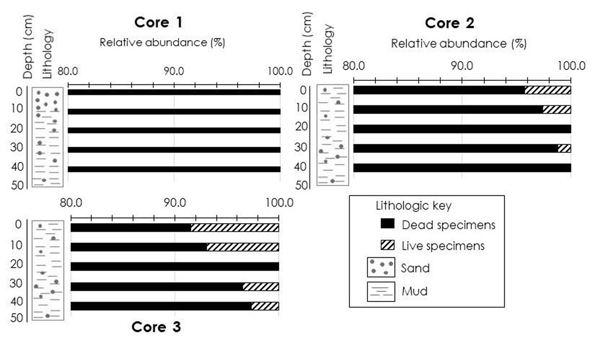
Figure 3
Relative abundance of dead and live foraminiferal assemblages in all cores taken at three locations in the Kemaman-Chukai mangrove swamp.
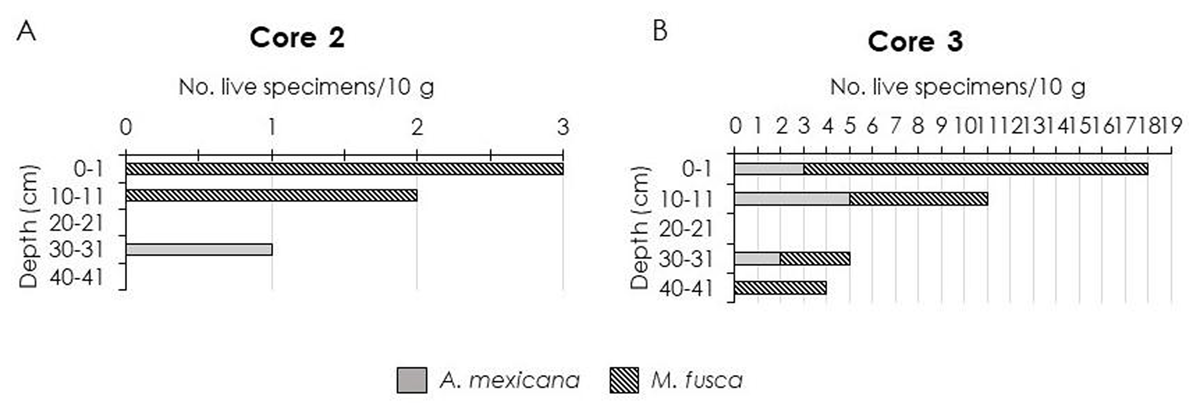
Figure 4
A and B showing number of live specimens/10 g of sediment throughout the cores.
Core 3 (Landward Core)
Muddy sediment was observed throughout the core but sandier in the 30–31 cm interval (Table 1). Salinity was 28 ppt and elevation level was 1.2 m (MSL). Mangrove vegetation was dominated by Xylocarpus granatum and Nypa fruticans. TOC ranged between 5.7–5.9 and no crab mounds were observed in this coring site.
In comparison, the number of dead and live foraminifera in Core 3 were higher than recorded in Core 1 and 2 (Figure 3). Number of dead specimens/10 g of sediment were much higher (95%) than numbers of live foraminifera (5%) (Figure 3). The highest number of dead foraminifera was recorded in the 0–1 cm interval (194 specimens/10 g of sediment) and decreased down-core.
A notable increase in the number of live foraminifera was observed in Core 3 and they were found down to the 40–41 cm interval (Figure 3). Peak concentrations of living foraminiferal populations occurred in upper 1 cm sediment (18 specimens/10 g of sediment) and later decreased down-core (Figure 3). Similar to Core 2, only Arenoparrella mexicana and Miliammina fusca were found living infaunally in the sediment (Figure 4). S values varied from 10–14 in dead foraminifera and 2 in live foraminifera; α values ranged from 2.4–3.8 in dead foraminifera and 0.6–1.2 in live foraminifera; H’ values recorded from 1.2–1.8 in dead foraminifera and 0.5–0.7 in live foraminifera; J’ values ranged from 0.5–0.7 in dead foraminifera and 0.7–1 in live foraminifera (Table 1). Seventeen taxa were recorded, mainly dominated by Arenoparrella mexicana, followed by Haplophragmoides wilberti and Miliammina fusca (Table 2). Scanning Electron Microscope (SEM) images of some dominant taxa are illustrated in Figure 5.
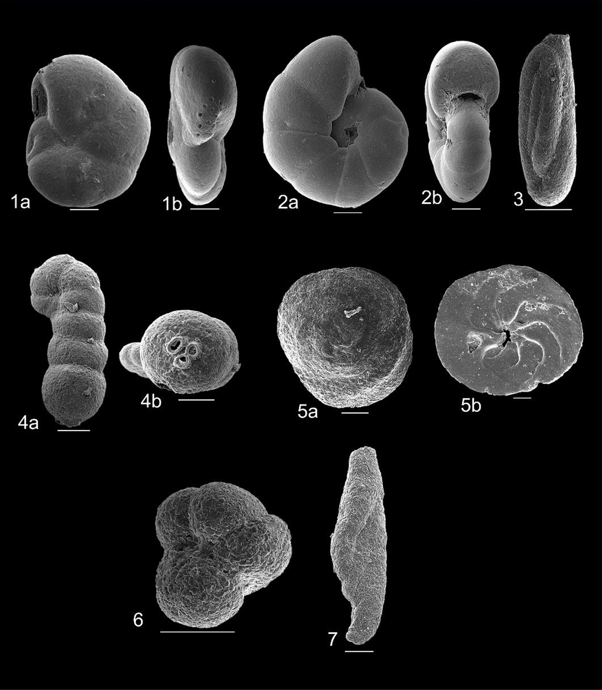
Figure 5
Scanning Electron Microscope images of some foraminiferal species identified from Kemaman-Chukai mangroves. Scale bars = 100 μm. 1 = Arenoparrella mexicana (Kornfeld, 1931) a) ventral b) side; 2 = Haplophragmoides wilberti (Andersen, 1953) a) dorsal b) side; 3 = Miliammina fusca (Brady, 1870); 4 = Acupeina triperforata (Millett, 1899) a) side b) aperture; 5 = Bruneica clypea (Brönnimann, Keij and Zaninetti, 1983) a) dorsal b) ventral; 6 = Paratrochammina sp. (Brönnimann, 1979, emended Brönnimann and Whittaker, 1986); 7 = Ammotium pseudocassis (Cushman and Brönnimann, 1948).
Discussion
Spatial and Vertical Distribution Patterns of Foraminifera
Total population of foraminifera (dead and live) were low in the seaward core (Core 1) and higher at the two cores (Cores 2 and 3) from the more inland sites (Tables 1, 2; Figure 3). Core 1 located closer to the high wave energy of the South China Sea and with relatively high salinity (32 ppt), was dominated by sandy deposits. Intense environmental stress at this site may destroy most tests and reduce the number of living individuals especially in the 0–1 cm sample. This environment was not favourable for agglutinated foraminifera to flourish, thus resulting in a very low abundance of common mangrove taxa throughout the core (e.g., Arenoparrella mexicana and Miliammina fusca). Even though Core 1 is located at a site closer to the sea with high salinity, there were no calcareous taxa recorded either.
The transition between the front (Core 1) and middle and high mangrove (Core 2 and 3) corresponds to an increase in the relative abundance of the most dominant taxa; Arenoparrella mexicana, Haplophragmoides wilberti and Miliammina fusca. In Core 2 and 3, Arenoparrella mexicana consistently dominated the assemblages (relative abundance >40% at all intervals, except in Core 2, at 20–21 cm interval). In Core 3, the agglutinated species were represented by a more diverse assemblage compared to Core 2 despite having similar salinity range and sediment characteristics (but lower elevation was observed in Core 3; 1.2 m MSL and 2.0 m MSL in Core 2). Acupeina triperforata, Ammotium pseudocassis, Ammoastuta salsa and Trochammina spp. were among taxa with higher number of specimens recorded in Core 3 but low in Core 2.
Generally, the distributions of intertidal foraminifera can be divided into two zonations, 1) calcareous assemblage that dominates the mudflats and sandflats of the intertidal zone and 2) agglutinated assemblage that is distributed in the vegetated marsh (Horton et al. 2005). These zonations were formed as direct function of elevation, with the duration and frequency of intertidal exposure as the most crucial environmental factors (Horton et al. 2005). Arenoparrella mexicana, Miliammina fusca, Trochammina inflata, Ammobaculites exiguus, Haplophragmoides wilberti, Caronia exilis and Bruneica clypea were among agglutinated taxa observed in the landward margins of salt marsh and mangrove swamps worldwide (Horton et al. 2005; Murray, 2006; Berkeley et al. 2008; Culver et al. 2013). Assemblages dominated by Caronia exilis, Siphotrochammina lobata, Ammotium directum, and Ammobaculites exiguus, were recorded by Culver et al. (2013) in the high swamp of Setiu estuary and lagoon, Malaysia. Horton et al. (2005) identified high abundances of Arenoparrella mexicana, Miliammina fusca, Miliammina obliqua and Trochammina inflata at the landward edge of the mangroves of Kadelupa, Indonesia.
Infaunal Foraminifera and Microhabitats in the Kemaman-Chukai Mangrove
The number of infaunal foraminifera in this study varied according to depth in the cores analysed, as well as between cores and contributed only slightly (relative abundance) to the total assemblage; 0% in Core 1; 2% in Core 2; and 5% in Core 3. Only two out of eighteen taxa were observed living in the infaunal habitat (Arenoparrella mexicana and Miliammina fusca) with very low abundances (Figure 4).
Diversity values (number of specimens and species richness) were much lower compared to the adjacent mangrove of Setiu estuary and lagoon. Culver et al. (2013) reported nine taxa with >20 live specimens; Ammobaculites exiguus (95 specimens), Bruneica clypea (92), Siphotrochammina lobata (51), Arenoparrella mexicana (46), Caronia exilis (35), Trochammina inflata (29), Miliammina petila (25), Ammotium directum (23) and Haplophragmoides wilberti (22). In this study, only Miliammina fusca showed the highest number of live specimens; 33 specimens (Figure 4). This discrepancy may be resulted from different sample interval (2 cm in Culver et al. 2013 and 10 cm in the present study). Culver et al. (2013) also reported the deepest infaunal occurrence in Malaysia so far (78–80 cm depth interval, 11 specimens/20 cm3 of sediment) and was characterized by Bruneica clypea, Trochammina inflata and Siphotrochammina lobata.
Throughout the cores (Core 2 and 3), the abundance of infaunal foraminifera decreased with increasing depth (Table 2, Figure 3). The highest abundance of infaunal foraminifera was found in the upper 11 cm of Core 3, where they contributed 71.7% of the total infaunal population in this core. Even though the maximum depth where they were found alive (Rose Bengal stained) was at 40–41 cm (Core 3), their relative abundance in this interval constituted only 12.3% of the total infaunal population.
Infaunal foraminifera were found at sites with muddy (Core 2 and 3) rather than sandy sediments (Core 1) (Table 1). However, contrary to our results, Horton & Edwards (2006) reported a greater percentage of infaunal foraminifera in the sandier substrates of the tidal flat environment of Rusheen Bay, Ireland, with no occurrence of infaunal foraminifera were recorded in the high, middle and low marsh environments which was dominated by silty sediment. Berkeley et al. (2008) listed three important factors that contribute to the depths at which foraminifera can live: 1) sediment oxygenation – coarser substrates are associated with deeper oxygenated layer and therefore, favours the down-core distribution of infaunal foraminifera (Goldstein & Harben 1993); 2) bioturbation – by falling into tubes or burrows (Green, Aller & Aller 1993) or by deep burrowing activity of foraminifera to avoid predation e.g., crustaceans, gastropods, polychaetes (Lipps 1983); and 3) organic matter flux – food source for foraminifera. In this regard, the presence of infaunal foraminifera in Core 3 (with muddy sediment and less crab mounds observed) may be a response to organic matter availability rather than sediment oxygenation and bioturbation. On the other hand, no live/infaunal foraminifera occurrences in Core 1 may be resulted from bioturbation process by fiddler/mangrove crabs as observed from intense crab mounds in the surrounding area. Similar results have been observed in Bombay Hook marshes, USA where low abundances of infaunal foraminifera were observed in areas with extensive crab mounds (Leorri, Horton & Cearreta 2008).
Even though the abundance of infaunal foraminifera in the study area decreased with increasing depth, they were found to live deeper at the upper/landward mangrove site (Core 3) and shallower in the site closer to the sea (Core 2) (Figures 3 and 4). These microhabitat preferences correspond well with those found in the tropical intertidal environment of Cocoa Creek, Queensland, Australia (Berkeley et al. 2008) where species observed living in the distal mangrove area had deeper living habits than those found in the proximal mangrove and mudflat sediments.
More than 50% of the total population of infaunal foraminifera in Core 2 and 3 were found in the upper 11 cm of the core (Figures 3 and 4). Thus, foraminifera living in the 0–11 cm interval are considered to be shallow infaunal and those dwelling deeper than 11 cm are considered to be deep infaunal. This classification was based upon Culver & Horton (2005); and Leorri & Martin (2009). In the Setiu estuary and lagoon (Culver et al. 2013), shallow infaunal foraminifera were described as those living in the 0–16 cm interval, slightly deeper than this present study.
Bioturbation and Taphonomic Inferences
Foraminifera represent an important potential food source for many organisms, including flatworms, polychaetes, gastropods, bivalves and crustaceans because they are commonly present in great abundance in the water column, on the sea floor (Culver & Lipps 2003) and in the sediment (including mangrove-fringed estuary) (Stoner and Zimmerman, 1988). Predatory activities by these organisms undoubtedly causes taphonomic changes in foraminiferal assemblages as they fossilize and it varies from environment to environment (Culver & Lipps 2003).
Core 1 displayed significant evidence of bioturbation processes. Intense crab mounds at this site defined active predation by mangrove/fiddler crabs and increased the possibility of reworked sediment (by crabs burrowing deep into the sediment). In Core 2, the abundance of foraminifera at 20–21 cm depth was surprisingly low compared to super- and sub-jacent horizons (Figure 3). This could be a result of taphonomic removal of many of the foraminifera originally dwelling at that site at the time of sediment accumulation. It could also result from increased sedimentation rate possibly related to a major runoff event or storm surge. Thus, further study is suggested to understand the possible reasons behind the taphonomic loss of foraminifera in this study area, especially from this specific depth interval.
Comparison between distribution of live population and dead assemblages of foraminifera provides insights into the taphonomic loss of foraminiferal specimens (Culver et al. 2013). In landward core (Core 3), numbers of live specimens/10 g of sediment decreased down-core (Table 1 and Figure 4), but the numbers of dead specimens were high throughout the core length (despite the down-core percentage of dead specimens was reduced by 6% in the 10–11 cm interval) (Table 1). Below 11 cm, the relative abundance of dead assemblages remained consistent (97–100%) (Figure 3). Similar taxa (Arenoparrella mexicana, Haplophragmoides wilberti and Miliammina fusca) characterized the upper 1 cm and subsurface assemblages. This pattern, suggesting less taphonomic loss down core compared to seaward (Core 1) and middle core (Core 2). Although the number of Miliammina fusca (specimens/10 g of sediment) was irregular down core (Table 2), this patchiness was compensated by increased number of specimens of Haplophragmoides wilberti. This pattern was believed to be an environmentally driven assemblage change rather than taphonomic activity (Culver et al. 2013).
The preservation potential of Miliammina fusca in the core of this present study was in contrast to the Setiu estuary and lagoon, Malaysia (Culver et al. 2013). Generally, Miliammina fusca was listed as one of the taxa that are less likely to be preserved. The non-mineralized, organic cement of the test of Miliammina fusca make them susceptible to degradation (Lipps 1971). In Setiu estuary and lagoon samples (e.g., SET10 SET1), two dead specimens of Miliammina fusca/20 cm3 of sediment was recorded from 38–40 cm interval but our result showed better preservation (21 specimens/10 g of sediment in the 40–41 cm interval) (Figure 3).
Implications for Sea-Level Reconstructions
Foraminifera have been an excellent biological proxy in evaluating the significance of recent changes in relative sea-level, since they are capable of bridging the gap between short instrumental records (e.g., tide gauges) and longer term geological data (Shennan et al. 2015; Edwards & Wright 2015). Spatial variability in the composition, elevation and vertical range of foraminiferal zonation provides fundamental constraints on the application of an assemblage zone approach to the reconstruction of former relative sea-level (Horton & Edwards 2006).
In this study, distribution patterns of subsurface and infaunal foraminifera in the Kemaman-Chukai mangrove swamps differ from core to core. In seaward core (Core 1 with extensive crab mounds), numbers of dead foraminifera were very low and inconsistent throughout the core, with no infaunal foraminifera were observed, indicating intense bioturbation by mangrove crabs. In Core 2 (middle core), even though the numbers of live foraminifera decreased down core, the number of dead specimens were inconsistent especially in the 20–21 cm interval, indicating taphonomic loss of specimens. Core 3 (landward core) however, displayed an ideal foraminiferal distribution patterns required in the palaeo sea-level reconstruction (with less taphonomic loss and decreasing number of infaunal foraminifera down core).
Our results derived from Core 3 resemble those from the mangrove of Setiu estuary and lagoon (Culver et al. 2013). Based on a comparison with the Setiu estuary and lagoon data, the dead assemblage in this present study was formed in the 0–11 cm interval, slightly shallower than the two Setiu high-swamp cores. This interval was thin enough to produce multi-decadal to centennial-scale temporal resolution reconstructions (which equivalent to C-14 age resolution), based on the Pb-210 derived sedimentation rate of ~0.3 cm yr–1 (Culver et al. 2013). Because of the similarity displayed in the foraminiferal assemblages in the 0–1 cm and 10–11 cm intervals, surface sample (0–1 cm) should be an acceptable basis (Culver et al. 2013) for down core reconstructions in this present study.
Conclusion
Agglutinated taxa dominated our samples with no records of calcareous foraminifera. In general, species found in this present study were common and similar with mangrove foraminifera worldwide. Bioturbation and taphonomic loss were intense in seaward (Core 1) and middle core (Core 2). High-mangrove-swamp core (Core 3) was proven to be the optimum site for sea-level or palaeoenvironmental research in this region and is in agreement with other infaunal foraminiferal study from Malaysian mangrove swamps.
Additional File
The additional file for this article can be found as follows:
Lay Summary
Mangrove foraminifera as a key to the past sea-level. DOI: https://doi.org/10.5334/oq.95.s1
Acknowledgements
We thank the Institute of Oceanography and Environment (INOS) staff for providing technical support, Kemaman Forestry Department, and postgraduate comrades for their help in the field. We also thank Prof. Dr. Stephen Culver from East Carolina University who kindly assisted us with foraminiferal identification and manuscript revision.
Funding Information
This project was funded by the Higher Institute Centre of Excellence (HICoE) Grant (Vote No. 66928) awarded to Institute of Oceanography and Environment (INOS), Universiti Malaysia Terengganu and Fundamental Research Grant Scheme (FRGS/1/2018/WAB09/UMT/02/3) provided by Ministry of Higher Education Malaysia.
Competing Interests
The authors have no competing interests to declare.