
1. Introduction
Being the largest convective area on Earth, the Asian monsoon plays a crucial role in the global climate system by transferring heat energy and humidity from the equator to the higher latitudes (e.g., Webster et al. 1998; An et al. 2000; Zahn, 2003; Pausata et al. 2011; Cook & Jones 2012; Chabangborn et al. 2014; Chabangborn & Wohlfarth 2014; Jo et al. 2014). With seasonal wind reversals driven by a complex interaction of the land-sea thermal contrasts, monsoonal regions are characterised by heavy summer rainfall and relatively dry winters. Studies have shown that large-scale atmospheric mechanisms such as the El Nino Southern oscillations (ENSO) -expressed as El Niño, with drier conditions in Mainland Southeast Asia (MSEA), and La Niña, with enhanced rainfall in the region- and the mean shift of intertropical convergence zone (ITCZ) modulates tropical monsoonal rainfall (e.g., Yamoah et al. 2021).
MSEA is situated near the boundary of the Asian monsoon system, which includes the Indian Ocean and East Asian monsoon sub-systems (Wang et al. 2003; Wang et al. 2005; Chabangborn & Wohlfarth 2014). As a result, MSEA is regarded as a crucial location for understanding the variability of the Asian monsoon (Cook & Jones 2012; Chabangborn & Wohlfarth, 2014). Consequently, the distinctive change in MSEA paleo-coastline, particularly the exposure of the Sunda Shelf during the Last Glacial Maximum (LGM), can influence the global-scale atmospheric circulations.
The LGM saw a decrease in global temperatures and advance of the continental ice sheets extending between 26.5 and 20 cal ka BP (e.g., Clark et al. 2009). The expansion of the ice sheets affected the position and strength of the jet streams subsequently impacting the monsoonal flow, disrupting the regular circulation patterns, and contributing to a weaker monsoon. In addition, this led to cooler sea surface temperatures (SSTs) in tropical and subtropical oceans. The altered SST gradients and atmospheric circulation patterns during the LGM, especially in the Tropical Pacific Ocean, could have impacted the occurrence and characteristics of ENSO events, which modulates the monsoon variability (Koutavas & Lynch-Stieglitz, 2003; Loo et al. 2015). Furthermore, during this period, the lower atmospheric CO2 concentrations would not only have contributed to the overall cooler climate but also influenced vegetation cover and land surface properties (Yasunari 2007; Beerling & Royer 2011).
Meanwhile, the expansion of the ice sheet made the sea level fall to approximately 125 m below the mean sea level (BMSL) (e.g., Bird et al. 2005; Hanebuth et al. 2011; Raes et al. 2014). The Sunda shelf was exposed, connecting MSEA and the Indonesian archipelagos known as the Sundalnd (e.g., Bird et al. 2005; Raes et al. 2014). The paleo-coastline extended eastward from the Thai-Malay Peninsular to the South China Sea. The emergence of the Sunda Shelf during the LGM significantly affected the hydroclimate conditions of the western Pacific Warm Pool (Webster 1994; Trenberth et al. 1998; Bush & Fairbanks 2003).
Studies by Quinn (1971), Hostetler & Mix (1999), Bush & Fairbanks (2003), and Partin et al. (2007) suggest that the emergence of Sundaland enhanced the Pacific walker circulation (PWC), creating conditions similar to present-day La Niña-like conditions. Other studies have also suggested a weaker monsoon during this period as a result of reduced solar insolation (Wang et al. 2003). The reduced insolation likely impacted the differential heating of the land and the ocean -land-sea thermal contrast- thus leading to weakened summer monsoon rains across Southeast Asia (Li & Yanai 1996; Wang et al. 2003; An et al. 2015). Similarly, Wurster et al. (2019) showed forest contraction in peninsular Malaysia and Palawan during the LGM, indicating generally drier conditions.
The inconsistencies among proxy records (e.g., An et al. 2015; Wurster 2019) are further complicated by the ambiguity associated with LGM climate simulations in the MSEA (De Deckker et al. 2002; Di Nezio & Tierney 2013; Chabangborn et al. 2014; Sarr et al. 2019; Tian 2024). Therefore, this study aims to analyse sedimentary records from the lower central plain of Thailand, which is situated near the northernmost part of the Sunda shelf, using a suite of proxies, including geochemical compositions, grain size, and pollen analysis. This approach seeks to enhance our understanding of the mechanisms driving hydroclimatic conditions in the MSEA region during the LGM.
2. Regional settings
The lower central plain of Thailand covers an area of approximately 36,000 km2 (Sinsakul 2000) (Figure 1a). This flat and low-lying region extends from the Chao Phraya River flowing southward in Chinat Province to the narrow strip of tidal flat and mangrove forest in the north of the Gulf of Thailand (Sinsakul 2000) (Figure 1b). Alluvial fans and terraces border the western and eastern margins of the plain. Elevations in the plain are around 15 m, 2.5 m, and 1.5 m above mean sea level (AMSL) in Chainat, Ayutthaya, and Bangkok, respectively, from north to south (Figure 1b).
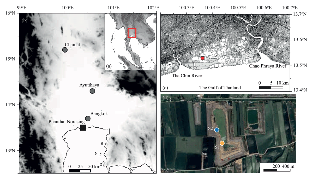
Figure 1
Location of the study area on (a) the lower central plain of Thailand (b) situated 1.5 km west of the Provincial Administrative Organisation of Phanthai Norasing sub-district in Samut Sakhon Province, 50 km west of Bangkok, and 5 km north of the upper Gulf of Thailand (red square) (c). The sediment samples were taken from an unnamed open excavation, covering an area of 0.42 km2 and approximately 24 m depth (d). The sampling sites were moved from S1 (orange circle) to S2 (blue circle) caused by the sediment slump along the open pit road.
The geology of the lower central plain consists of 2,000 m thick of Quaternary sediments overlaying the Tertiary rocks, including claystone, siltstone, sandstone, and conglomerate (Sinsakul 2000). However, studies of the Quaternary sediments have primarily focused on the late Pleistocene and Holocene epochs (approximately 300-600 m depth) due to limited information from shallow boreholes, open pits, and groundwater wells (Sinsakul 2000; Tanabe et al. 2003). The late Pleistocene sequences are characterized by sand and sand interbedded with clay and gravel, with stiff clay occasionally found on top. Iron and manganese pisolitic concretions and red and orange mottles in the stiff clay indicate subaerial conditions, reflecting alluvial and fluvial depositional environments during the late Pleistocene (Sinsakul 2000). The Holocene successions consist of dark grey silty clay, influenced mainly by fluvial processes in the northern plain and tidal processes due to relative sea-level fluctuations in the Gulf of Thailand in the south (e.g., Somboon 1988; Somboon & Thiramongkol 1992; Tanabe et al. 2003; Punwong 2007; Songtham et al. 2007; Negri 2009; Hutangkura 2012; 2014; Songtham et al. 2015).
For this study, sediment samples were collected from an unnamed open pit with an area of 0.42 km2 and a depth of approximately 24 m, located at 1.18 m AMSL according to Differential Global Positioning System (DGPS) measurements (Figures 1c and 1d). The pit is situated 1.5 km west of the Provincial Administrative Organisation of Phanthai Norasing sub-district in Samut Sakhon Province, 50 km west of Bangkok, and 5 km north of the upper Gulf of Thailand (Figure 1c). This coastal plain lies between the Tha Chin and Chao Phraya Rivers, in the southern part of the lower central plain of Thailand (Figure 1c). The highest tide reaches 1.71 m AMSL and can rise to 2.7 m AMSL during storm surges (Arends et al. 2016). Despite being fringed by prawn farms, salt ponds, factories, and shelters, mangrove forests thrive along the Tha Chin estuary and riverbank (Meepol et al. 1997).
The Asian monsoon significantly influences Thailand’s climate (e.g., Wohlfarth et al. 2012; Chabangborn et al. 2020; Jirapinyakul et al. 2023). The southwest monsoon brings humid air from the Indian Ocean, increasing precipitation from mid-May to October. From November through February, the northeast monsoon predominates, leading to cold and dry weather. High temperatures and humidity prevail from February to May due to the high sun and southerly and south-easterly breezes. Samut Sakhon receives an annual precipitation of 1200 to 1400 mm (Thai Meteorological Department 2023), with September experiencing the highest rainfall, ranging between 200 and 300 mm. The mean annual temperature is between 28 and 30°C.
3. Methodology
The lithological succession of the open pit was described from bottom to top during a field investigation in April 2022. Sediment samples were collected approximately every 10 cm by hammering PVC pipes, 2 cm in diameter and 10 cm long, into the sediments. Additional 2 cm thick samples were collected 30 cm from the sampling point and stored in plastic zip lock bags for radiocarbon dating. The sampling locations were relocated from S1 to S2 due to the sediment slump along the open pit road (Figure 1d). A total of 73 samples were taken from depths ranging from approximately 24.3 to 16.2 m BMSL. The reference depths were verified using a laser level-measuring telescope and DGPS measurements.
All the samples were then transported and stored in a refrigerator at the Department of Geology, Faculty of Science, Chulalongkorn University, for further analysis, including X-ray fluorescence (XRF), loss on ignition (LOI), grain size distribution, pollen analysis, and radiocarbon sample preparation.
The samples were dried at 105°C for 12 hours, ground, and homogenised. Each dried sample was placed in a plastic crucible and wrapped with a 4 µm thick prolene film to prevent direct contact with the XRF measurement window. Geochemical compositions of the sediments were measured using a portable Olympus Vanta XRF series, relying on Compton normalisation, for 3 minutes at the Department of Geology, Faculty of Science, Chulalongkorn University. The XRF detected the concentrations of 39 elements: P, S, Cl, K, Ca, Ti, V, Cr, Mn, Fe, Co, Ni, Cu, Zn, As, Se, Rb, Sr, Y, Zr, Nb, Mo, Ag, Cd, Sn, Sb, Ba, La, Ce, Pr, Nd, Ta, W, Au, Hg, Pb, Bi, Th, and U. However, concentrations of P, Cr, Co, Se, Mo, Ag, Cd, Sn, Sb, La, Ce, Pr, Nd, Ta, W, Au, Hg, Bi, Th, and U did not reach the detection limit, and concentrations of S, V, Mn, Ni, Cu, As, Se, and Y were missing in some data points. Therefore, these 29 elements were excluded from further analysis. Ultimately, the concentrations of Cl, K, Ca, Ti, Fe, Rb, Sr, Zr, Zn, and Ba were included in the correlation matrix to assess the relationships between each element (Supplementary 1).
After the XRF analysis, the dried samples were weighed and combusted at 550°C for 6 hours to assess organic matter content and at 950°C for 3 hours to determine carbonate content (Heiri et al. 2001; Wohlfarth et al. 2012). The loss on ignition (LOI) was calculated as the percentage weight loss of the dried sample.
For grain size analysis, the samples were treated with 20 ml of 10% (v/v) HCl to remove carbonates and with 20–10 ml of 30% (v/v) H2O2 to eliminate organic matter (Rowell 1994). The prepared samples were then sent to the Department of Marine Science, Faculty of Science, Chulalongkorn University, for grain size analysis using a Horiba LA-960V2 laser diffraction analyser. The results were subsequently analysed using the GRADISTAT program (Blott & Pye 2001). To understand sediment transportation and depositional processes, we displayed the coarse (one percentile) and median (fifty percentile) diameters of the sediments in the CM diagram (Passega 1964; Kasim et al. 2023; Miao et al. 2023).
The selected geochemical compositions (as detailed in the results and discussions) and grain size analysis from the sedimentary succession were eventually compared with those of the recent sediment obtained by Hossain et al. (2017), corrected by sediment transport volumes in Chao Phraya and Tha Chin Rivers as reported by Park et al. (2021).
One cubic of sixteen samples were taken at 50–30 cm intervals for pollen analysis, representing each sediment unit. These samples were sieved with a 0.2 mm mesh. Pollen and spores were extracted using acetolysis method the heavy liquid separation with sodium polytungstate (3Na2WO4•9WO3•H2O) (Englong et al. 2019). Afterwards, an aliquot of each treated sample was dried onto a coverslip and then mounted onto a glass slide. Pollen and spores from each depth interval were identified and counted under light microscopy using modern pollen reference at the Faculty of Environmental and Resource Studies, Mahidol University, and the Department of Geology, Faculty of Science, Chulalongkorn University. The samples aimed for a count of 150 pollen grains, but the pollen content in all samples was sparse and insufficient to achieve this target.
Neither plant remains nor charcoal were found in the samples. Consequently, bulk sediment samples were sent to DirectAMS for radiocarbon analysis using accelerator mass spectrometry (AMS). The 14C age ± one standard deviation (SD) was calculated following the conventions of Stuiver and Polach (1977) using a Libby half-life of 5568 years and a fractionation correction based on δ13C measured on the AMS. The radiocarbon dating results were calibrated with the Calib 8.0 online program using IntCal20 (Reimer et al. 2020), and an age-depth model was constructed by linear interpolating between the selected adjacent dating results.
4. Results
4.1 Lithostratigraphy, grain size analysis, and LOI
The sedimentary succession in the pit can be divided into four units (A to D) based on their physical properties (Figures 2 and 3a). The lowermost unit A consists of light grey clayey silt below 23.3 m BMSL (Figures 2a and 3a). Laser diffraction analysis indicates that unit A comprises 2–5% sand, 70–76% silt, and 21–28% clay (Figure 3b), with a median diameter of approximately 8 µm (Figure 3c). The LOI at 550°C and 950°C showed minimal changes, at 7.5% and 2%, respectively (Figures 3d and 3e). The CM diagram suggests that pelagic suspension (T) was the primary mode of sediment transport in unit A (Figure 4).
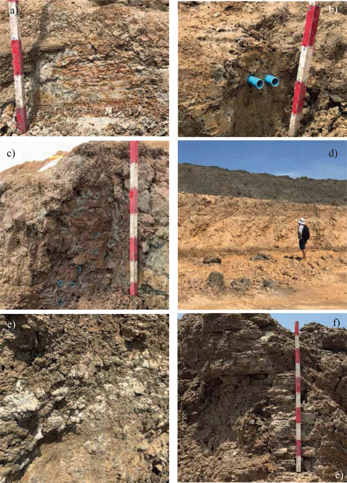
Figure 2
The lowermost unit A composes of light grey clayey silt (a). It is overlaid by unit B, consisting of interbedded clayey and sandy silt layers (b and c). Unit C is the thick bed of the brown silty sand (d), except for the brown silty sand with calcrete or caliche layer (e) from 18.6 to 18.2 meters BMSL. The uppermost unit D consists of thin beds (5–10 cm thick) of light grey clayey silt (f).
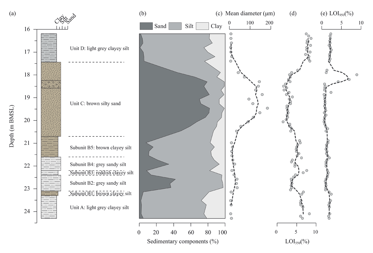
Figure 3
Lithostratigraphy (a), sedimentary compositions (b), mean diameter (c), and LOI at 550 (d) and 950°C (e). The back dash lines are moving average of five data points.
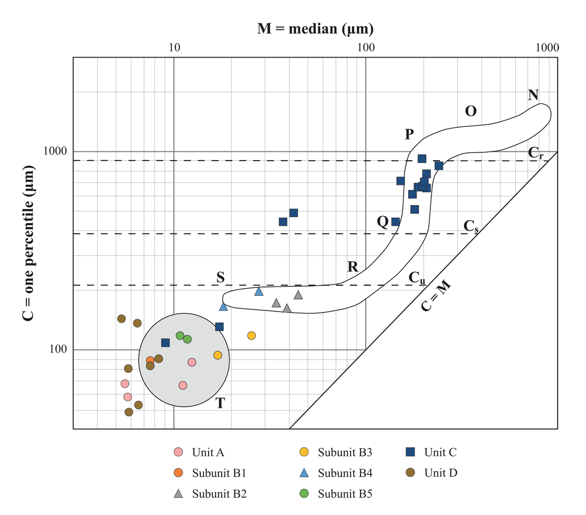
Figure 4
The coarse (C: one percentile) and median (M: fifty percentile) diameters of sediment were illustrated in the CM diagram to elucidate sediment transportation and depositional processes (Passega 1964; Kasim et al. 2023; Miao et al. 2023). According to the river and marine coastal sediment analysis, Passega and Byramjee (1969) established the transportation limits of rolling (Cr), graded suspension (Cs), and uniform suspension (Cu). The diagram is divided into five segments, corresponding points N, O, P, Q, R, S, and T. They consist of rolling (NO), bottom suspension and rolling (OPQ), graded suspension without rolling (QR), uniform suspension (RS), and pelagic suspension (T) (Kasim et al., 2023). The CM diagram demonstrates that pelagic suspension (T) plays a crucial role in the sediment transportation in the sedimentary units A and D, along with subunits B1, B3, and B5 (the circles). The sediment transportation mechanisms shift to uniform suspension (RS) in subunits B2 and B4 (the triangles), and suspension and rolling (PQ) in unit C (the squares), suggesting an increase in transportation energy.
Unit B, which spans from 23.3 to 20.7 m BMSL, consists of interbedded clayey and sandy silt layers and is divided into five subunits (B1 to B5) from bottom to top (Figures 2b, 2c, and 3a). Subunits B1 (23.3–23.1 m BMSL) and B5 (21.6–20.7 m BMSL) are composed of brown clayey silt (Figure 2b), while subunit B3 (22.4–22.2 m BMSL) is characterised by reddish clayey silt (Figure 3a). Laser diffraction results indicate that subunits B1, B3, and B5 consist of approximately 10% sand, 75% silt, and 15% clay (Figure 3b). Subunits B2 (23.1–22.4 m BMSL) and B4 (22.2–21.6 m BMSL) are characterised by grey and reddish sandy silt, containing a higher proportion of coarse grain fractions (Figures 2c and 3a). The sand fraction in subunits B2 and B4 averages 34%. In contrast, the silt and clay fractions decrease to 60% and 5%, respectively (Figure 3b). The median diameters in subunits B1, B3, and B5 range from 7 to 10 µm, whereas in subunits B2 and B4, they range from 20 to 35 µm (Figure 3c). The LOI at 550°C gradually decrease to 4% in subunits B1 and B2, increases to 6% in subunit B3, and shows insignificant changes ranging from 5% to 6% in subunits B3, B4, and B5 (Figure 3d). The LOI at 950°C remains constant in unit B and is comparable to that in unit A (Figure 3e). According to the CM diagram, sediment transportation processes shifted between pelagic suspension (T) in subunits B1, B3, and B5, and uniform suspension (RS) in subunits B2 and B4 (Figure 4). These results indicate changes in sediment transportation processes within unit B.
Unit B transitions gradually into the brown silty sand of Unit C, which spans from 20.7 to 17.4 m BMSL (Figures 2d and 3a). In Unit C, the sand content increases significantly from 50% to 80% (Figure 3b). In comparison, the silt and clay fractions decrease gradually to 40–20% and 10–5%, respectively (Figure 3b). The median diameter of the sediments increases sharply from 30 to 150 µm between 21.2 and 19.9 m BMSL, changes slightly from 19.9 to 18.3 m BMSL, and then drops abruptly to 40 µm from 18.3 to 17.9 m BMSL (Figure 3c). The LOI at 550°C decreases to approximately 2.5% before gradually increasing to 8% between 18 and 17.4 m BMSL (Figure 3d). The LOI at 950°C remains constant at around 2%, except from 18.6 to 18.2 m BMSL, which shows a significant increase to 10% (Figure 3e). The CM diagram indicates a shift in the sedimentary transportation mechanism to bottom suspension and rolling (OPQ), suggesting an increase in transportation energy in Unit C (Figure 4).
Within Unit C, there is an interval of brown silty sand with light grey gravel (approximately 10–25%) from 18.6 to 18.2 m BMSL, forming a massive horizon in some parts (Figures 2e and 3a). XRD analysis conducted at the Department of Geology, Faculty of Science, Chulalongkorn University, identified the gravel as calcium carbonate (CaCO3), indicating the presence of a calcrete or caliche layer (Wright 2003). Since there are no nearby limestone mountains, the CaCO3 layer is likely a secondary sedimentary structure formed by leaching through shell fragments above, transportation in solution, and reprecipitation at the groundwater table.
Unit D consists of thin beds (5–10 cm thick) of light grey clayey silt found between 17.42 and 16.22 m BMSL (Figures 2f and 3a). The sedimentary components and mean diameter in Unit D are similar to those in the lowermost Unit A (Figures 3b and 3c). The LOI at 550°C and 950°C are stable at 8% and 2.5%, respectively (Figures 3d and 3e). The CM diagram shows that the transportation process in Unit D is characterised by pelagic suspension (T) (Figure 4).
4.2 Geochemistry
For the down core, the XRF analysis shows that Fe is the most predominant element in the sedimentary sequence with a concentration of 32,300 ppm, followed by 13,400 ppm of K, 9,300 ppm of Cl, and 3,200 ppm of Ti (Figures 5b, 5c, 5d, and 5e). Trace amounts of Ba, Zr, Rb, Sr, and Zn are present at average concentrations of 374, 270, 125, 97, and 51 ppm, respectively (Figures 5g, 5h, 5i, 5j, and 5k).
The concentrations of Fe, K, Ti, Rb, and Zn display similar variation patterns (Figures 5b, 5c, 5e, 5i, and 5k). In units A and B1, these elements increase, reaching approximately 40,000 ppm for Fe, 15,000 ppm for K, 4,200 ppm for Ti, 170 ppm for Rb, and 70 ppm for Zn. Their concentrations decrease in units B2 to B4, then increase again in unit B5. In unit C, the Fe, K, Ti, Rb, and Zn concentrations drop to around 25,000, 10,000, 1,500, 100, and 25 ppm, respectively, before gradually increasing in the upper part of units C and D (Figures 5b, 5c, 5e, 5i, and 5k).
The concentration of Cl gradually declines from approximately 10,000 ppm in unit A to 2,000 ppm in unit D, with abrupt increases at depths of 22.2 and 19 m BMSL (Figure 5d). Ca concentrations range from 1,000 to 2,000 ppm in units A, B, and the lower part of unit C (approximately 20.5 to 18.6 m BMSL) (Figure 5f). In the caliche layer (approximately 18.4 to 18 m BMSL), Ca concentration spikes to 150,000 ppm before decreasing to 200–500 ppm in the upper part of unit C and unit D (approximately 18 to 17.4 m BMSL) (Figures 5a and 5f).
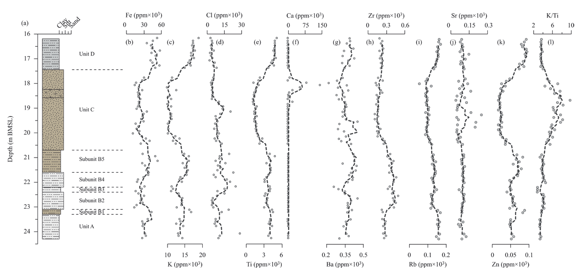
Figure 5
Lithostratigraphy (a), the variation of Fe (b), K (c), Cl (d), Ti (e), Ca (f), Ba (g), Zr (h), Rb (i), Sr (j), and Zn (k) concentrations, as well as the K/Ti ratios (l). The back dash lines are moving average of five data points.
Ba concentration gradually increases from 300 to 450 ppm in units A and B but is interrupted by a depletion in subunit B3 (Figure 5g). Ba concentration decreases in unit C before gradually increasing again in unit D. Zr concentration rises sharply from 250 ppm in unit A to 400 ppm in subunit B2 (Figure 5h), then gradually declines to 180 ppm in subunits B3 to B5 before slightly increasing to 250 ppm in units C and D. Sr concentration varies between 55 and 100 ppm, progressively increasing from units A to D, except for a depletion observed in unit C (Figure 5j).
The concentrations of Fe, Zn, and Ba in the sediment sequence are comparable to those found in recent sediment samples from the Chao Phraya and Tha Chin Rivers (Wijaya et al. 2013; Hossain et al. 2017; Asokbunyarat & Sirivithayapakorn 2020). However, the average concentrations of Sr and Zr are higher in the sediment sequence than in recent sediments, while K, Ti, and Rb concentrations are lower (Hossain et al. 2017). The calcium concentration in the sediment sequences is similar to that in recent sediments, except for a significant increase in the caliche layer, reaching a maximum of 150,000 ppm (Figures 5a and 5f). This supports the idea that the caliche layer is a secondary sedimentary structure formed by the leaching of CaCO3 from the upper sedimentary layers. Consequently, Ca concentration is excluded from the correlation matrix (Table 1).
Table 1
The correlation metric assesses the relationship between the concentrations of geochemical components within the sedimentary sequence. The grey highlights indicate the strong correlation of r values over 0.7. The p-values are below 0.001, indicating statistical significance.
| Cl | K | Ti | Fe | Zn | Rb | Sr | Zr | Ba | |
|---|---|---|---|---|---|---|---|---|---|
| Cl | 1.00 | ||||||||
| K | –0.11 | 1.00 | |||||||
| Ti | 0.01 | 0.91 | 1.00 | ||||||
| Fe | –0.04 | 0.75 | 0.67 | 1.00 | |||||
| Zn | –0.08 | 0.95 | 0.93 | 0.80 | 1.00 | ||||
| Rb | 0.09 | 0.82 | 0.92 | 0.59 | 0.81 | 1.00 | |||
| Sr | 0.11 | 0.00 | –0.04 | 0.08 | 0.07 | –0.05 | 1.00 | ||
| Zr | 0.21 | 0.37 | 0.47 | 0.01 | 0.38 | 0.35 | –0.02 | 1.00 | |
| Ba | 0.00 | 0.28 | 0.22 | 0.15 | 0.27 | 0.18 | 0.35 | 0.18 | 1.00 |
The correlation matrix shows a significant positive relationship (p-values < 0.001) among Fe, K, Ti, Rb, and Zn (Table 1). Iron-bearing minerals can be transported as detrital particles via wind or water (Williamson 1999). Ferrous iron released by chemical weathering readily oxidizes to form ferric oxides, which can either form a discrete phase or coat other solids present as detritus (Williamson 1999). In sedimentary processes, K concentration is influenced by the intensity of chemical weathering (Gaillardet et al. 1999; Grygar et al. 2019). Ti is abundant on the Earth’s surface as Ti-oxides, such as rutile and ilmenite, which are resistant to weathering and transportation (Yancheva et al. 2007; Löwemark et al. 2011; Kylander et al. 2011; Chawchai et al. 2016). Rb and Zn are prevalent in sedimentary processes through sorption and adsorption to clay minerals transported by rivers (Kylander et al. 2011; Wijaya et al. 2013; Asokbunyarat & Sirivithayapakorn 2020). These findings suggest that fluvial processes are likely the main factor influencing the Fe, K, Ti, Rb, and Zn concentration in the studied area. The intensity of chemical weathering has been subsequently conducted to enhance comprehension on the hydroclimatic shift.
Although chemical weathering is a primary factor influencing K concentration in sediments, other factors such as sedimentary provenance, pore water mineralization, and K-metasomatism may also play a role (Grygar et al. 2019). To reduce these uncertainties, immobile elements like Ti, Al, and Rb are often used to normalize K concentrations (Grygar et al. 2019). Since the K/Rb ratio reflects metasomatism, the K/Ti ratio is utilized here to assess chemical weathering variability (Grygar et al. 2019). The K/Ti ratio increases from 3.4 to 4.0 in units A to B2, decreases to 2.8 in unit B3, and ranges from 4.6 to 3.8 in units B4 to B5 (Figure 5l). The ratio significantly increases from 5.5 to 8.5 in unit C before showing a slight variation around 3.5 in unit D (Figure 5l).
4.3 Pollen analysis
The pollen content in this sediment sequence was sparse, ranging from 2 to 17 pollen grains. Subunits B1, B4–B5, and unit C were barren zones of pollen (Figure 6). In unit A, pollen of Suaeda (a hypersaline back mangrove herb) and Poaceae were found (Figure 6). In unit B2, Suaeda pollen significantly increased, reaching a maximum of 17 pollen grains (Figure 6). Pollen of Bruguiera (a landward mangrove species) and Poaceae were present in subunit B3. In unit D, only two pollen grains from Poaceae were identified (Figure 6). The scanty pollen and low LOI values at 550°C likely indicate the oxidation of organic compounds in an aerobic environment, suggesting a general exposure of a floodplain environment in the lower central plain (Figures 6 and 3d).
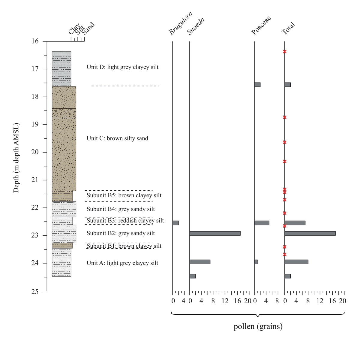
Figure 6
Lithostratigraphy and pollen stratigraphy. The red crosses are the sample that pollen is indeterminable.
4.4 Chronology
Since plant remains (e.g., leaves, charcoal, small twigs) were indeterminable, the chronology of the sedimentary succession relied on sequential radiocarbon dating of bulk sediments. This method is often subject to contamination by reworked older or younger organic materials (e.g., Björck & Wohlfarth 2001; Strunk et al. 2020). The dating results from samples D-AMS 048747, 050258, and 050259 showed significant inconsistencies with those from adjacent depths (Table 2).
Table 2
14C dates for the sediment sequence. Calibration of 14C dates is according to Reimer et al. (2020) and was made with the Calib 8.2 online program (http://calib.org/calib/calib.html). * are radiocarbon dating samples excluded in the age-depth plot in Figure 7.
| LAB CODE | SAMPLE TYPE | FRACTION OF MODERN | RADIOCARBON AGE (KA BP) | DEPTH (M BMSL) | 2-SIGMA (CAL KA BP) | MEDIAN (CAL KA BP) | ||
|---|---|---|---|---|---|---|---|---|
| pMC | ERROR | BP 1 | ERROR | |||||
| D-AMS 050257 | Bulk sediment | 6.291 | 0.08 | 22.22 | 0.102 | 24.32 | 26.11–26.92 | 26.51 |
| D-AMS 048747* | Bulk sediment | 16.85 | 0.13 | 14.31 | 0.062 | 24.30 | 17.12–17.73 | 17.39 |
| D-AMS 050258* | Bulk sediment | 2.473 | 0.053 | 29.72 | 0.172 | 21.94 | 33.91–34.55 | 34.27 |
| D-AMS 048748 | Bulk sediment | 9.33 | 0.11 | 19.05 | 0.095 | 20.88 | 22.70–23.19 | 22.99 |
| D-AMS 050259* | Bulk sediment | 6.14 | 0.11 | 22.42 | 0.144 | 20.16 | 26.38–27.11 | 26.74 |
| D-AMS 050260 | Bulk sediment | 9.624 | 0.09 | 18.81 | 0.075 | 17.30 | 22.50–22.95 | 22.73 |
Sample D-AMS 048747 was excluded because its modern fraction was significantly higher than the other samples (Table 2). Radiocarbon dating of molluscan shells and shelly layers in nearby areas by Tanabe et al. (2003) and Negri (2009) yielded ages of approximately 35 ka BP, similar to sample D-AMS 050258 (Table 2). Since molluscan shells and shelly layers were not found in this sedimentary sequence, the dating result of sample D-AMS 050258 was likely unreliable and not included in the chronology of the sedimentary sequence. Furthermore, the radiocarbon date from sample D-AMS 050259, which was inconsistent with adjacent dating results (D-AMS 048748 and 050260), was also excluded from the chronology (Table 2).
Therefore, the age-depth model for the section from 25.50 to 18.50 m BMSL is based on linear interpolating the results from samples D-AMS 050257, 048748, and 050260 (Table 2 and Figure 7). The age of this sedimentary sequence ranges from 26.5 to 22.65 cal ka BP, corresponding to the Last Glacial Maximum (LGM: 26.5–20 ka BP) (Figure 7b) (e.g., Clark et al. 2009). The sedimentation rate is approximately 0.1 cm/year between 24.32 and 20.88 m BMSL and significantly increases to 1.42 cm/year between 20.88 and 16.22 m BMSL (Figure 7b). These changes align well with variations in sediment compositions and transportation processes, as indicated by the CM diagram (Figures 3b, 4, 7a, and 7b).
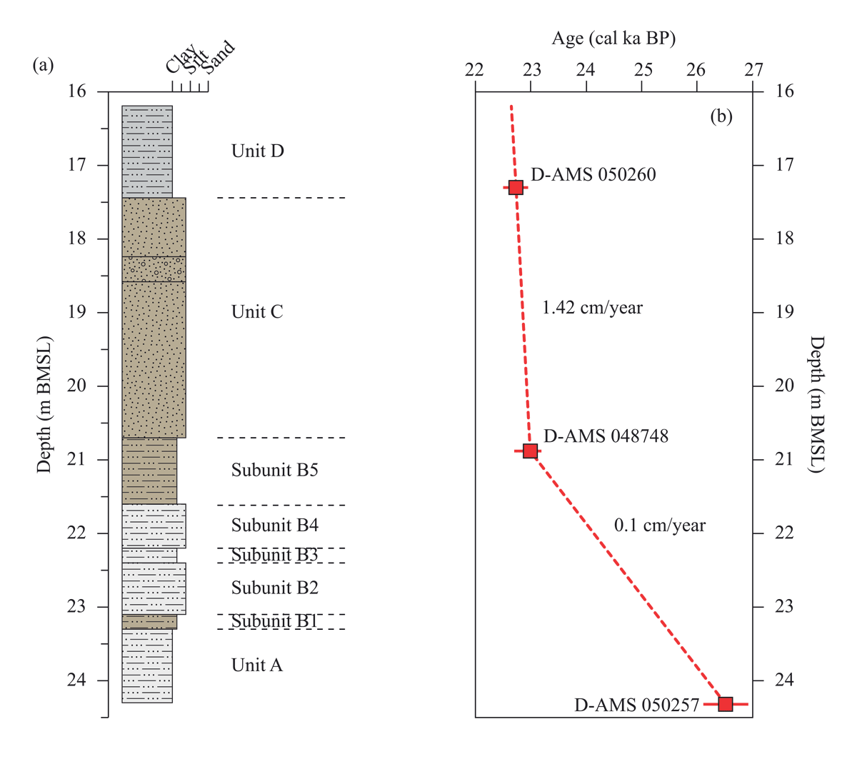
Figure 7
Lithostratigraphy (a) and the age-depth model (b) rely on three radiocarbon dating. The sedimentation rate is approximately 0.1 cm/year in units A and B and significantly increases to 1.42 cm/year in units C and D.
5. Discussions
Although the geochemical composition of sediments offers significant insights into watershed processes and catchment hydrology, the implications are complicated (Bertrand et al. 2024; Molén 2024). Consequently, the hydroclimate assessments conducted here rely on the K/Ti ratios associated with the mean grain size and sedimentary constituents. The recent sediments from the study area reveal distinct geochemical and sedimentological characteristics when weighted by sediment transport volumes from both river systems (see Hossain et al., 2017; Park et al., 2021). The K/Ti ratio averaged 3.35, indicating a moderate input of weathered detrital material (Hossain et al., 2017; Park et al., 2021) (Figure 8a). Grain size analysis shows that sand and silt fractions constituted approximately 65% of the total sediment composition, with a mean grain size of 1.7 µm (Hossain et al., 2017; Park et al., 2021) (Figure 8b). These results are used as a representative baseline for interpreting the variation in the downcore and also assess the overall influence of fluvial inputs on sedimentation in the central plain. The results of the recent sediments are generally comparable to the values derived from the sedimentary sequence (Hossain et al., 2017; Park et al., 2021) (Figures 8a and 8b), indicating a slight difference in the hydroclimatic conditions in the lower central plain of Thailand between the present and the LGM (#23, this study) (Figure 10). In contrast, the dominance of Suaeda and Poaceae presumably suggests arid conditions (e.g., Penny 2001; Hait & Behling 2019). The inconsistencies can be elucidated by the distribution of patchy grassland, which aligns with the present savanna climate in MSEA (Ratnam et al. 2016; Suraprasit et al. 2021).
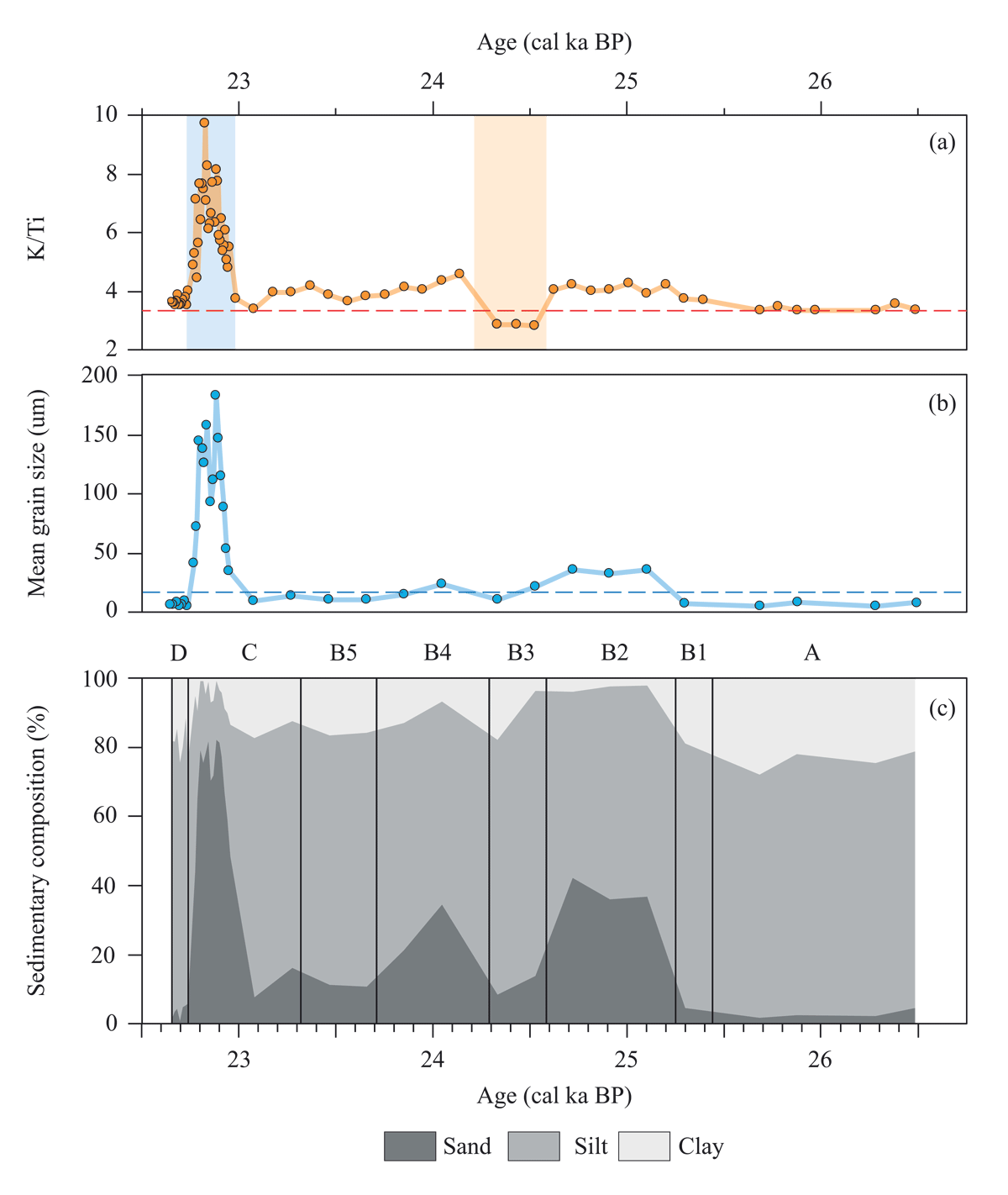
Figure 8
The sedimentary compositions, mean grain size, and the K/Ti ratios show the hydroclimatic change from 26.5 to 22.8 cal ka BP. The results indicate an intense runoff and increased rainfall from 26.5 to 24.6 cal ka BP, followed by a short period of drier conditions about 24.6–24.1 cal ka BP (red shading). Subsequently, there was a progressive decrease in the river runoff and precipitation until 23 cal ka BP, followed by notable wet conditions from 23–22.8 cal ka BP (blue shading). It was then terminated by a sudden lower runoff and precipitation after 22.8 cal ka BP. A comparison of the K/Ti ratio in recent sediment (red dash line) (Hossain et al., 2017) suggests that there may have been similar precipitation amount during the LGM and the present day.
Between approximately 26.5 and 24.6 cal ka BP, a gradual increase in fluvial runoff and precipitation was observed, as evidenced by a gradual rise in K/Ti ratios, mean grain size, and sand fraction (Figure 8). This period of wet conditions was followed by a brief phase of reduced discharge or lower precipitation between 24.6 and 24.1 cal ka BP, marking a significant shift in the climate (Figure 8). The drier interval may correspond to Heinrich Event 2 (23.6–24.4 cal ka BP, centred around 24 cal ka BP) (Hemming 2004; Cui et al. 2024). Following the wetter period, runoff and rainfall gradually declined from 24.1 to 23 cal ka BP (Figure 8). A significant increase in K/Ti ratios, mean grain size, and sand fraction between 23 and 22.8 cal ka BP points to a marked rise in river discharge driven by intensive precipitation (Figure 8). However, the climate took an abrupt turn after 22.8 cal ka BP, marked by sharp decreases in K/Ti ratios, mean grain size, and sand fraction, indicating a sudden and significant drying (Figure 8). These fluctuations are inconsistent with the conventional view of persistently cool and dry conditions associated with a weakened summer monsoon during the LGM in tropical regions (e.g., White et al. 2004; Cosford et al. 2010; Fleitmann et al. 2011).
Analysing the long-term trends in proxy records alongside datasets from MSEA provides insight into the atmospheric mechanisms that likely influenced the region’s hydroclimatic patterns during the LGM. In MSEA, our climatic reconstructions of a decrease in rainfall amount at 24.6–24.1 cal ka BP and a sharp increase in precipitation at 23–22.8 cal ka BP are ambiguous in the δ18O variability obtained from Hin Tum (#24) and Padamya (#25) (Liu et al. 2020) (Figures 9a, 9b, and 9c) (location in Table 3 and Figure 10). Interestingly, the δ18O records from Gunung Buda Cave, Borneo (#19; Partin et al. 2007), exhibit contrasting patterns during the same periods (Figures 9c and 9d) (location in Table 3 and Figure 10). These opposite variations may be linked to the southward and northward migration of the ITCZ at c. 24 and 23 cal ka BP. Alternatively, further comparisons of climatic records across the broader Pacific region suggest that ENSO-like phenomena potentially modulated tropical rainfall at 24 cal ka BP. δ18O records from El Condor Cave and Cueva del Diamante in the eastern Pacific reveal an increase in precipitation at about 24.5 ka (Figures 9e and 9f) (Cheng et al. 2013). These patterns contrast the drier conditions in the lower central plain of Thailand and Borneo during the same periods, indicating an El Niño-like phenomenon at 24 cal ka BP.
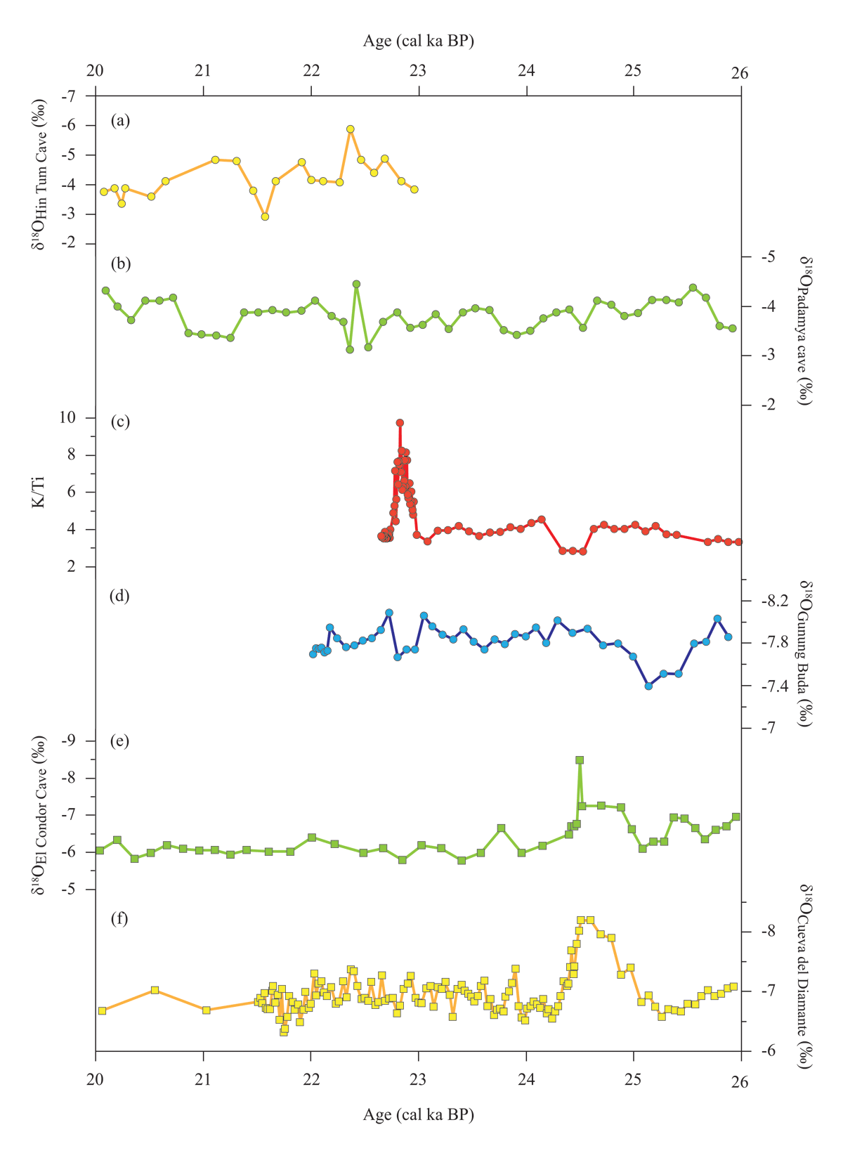
Figure 9
Comparison between the K/Ti ratios (c, red circles) and the δ18O values obtained from Hin Tum Cave (a, yellow circles), Padamya Cave (b, green circles), and Gunung Buda National Park (d, blue circles) in the western Pacific Ocean, and El Condor (e, green squares) and Cueva del Diamante Caves (f, yellow squares) in the eastern Pacific Ocean. Locations of the site in the east Pacific Ocean are shown in Figure 10 and Table 3. El Condor Cave is located 5.93°S and 77.3°W, while Cueva del Diamante is located at 5.73°S and 77.5°W.
Table 3
Palaeo-records and -proxies included in the compilation. The age assignments are determined using published 14C and U/Th dates. The number of dates within the time interval of 26–20 cal ka BP for each sequence is indicated in parentheses. See Figure 9 for the location of the sites.
| SITE NO. | SITE NAME | LAT (°) | LONG (°) | ELEVATION (M A.S.L.) | ARCHIVE | PROXY | AGE ASSIGNMENT | REFERENCES |
|---|---|---|---|---|---|---|---|---|
| 1 | GeoB10053-7 | –8.68 | 112.87 | –1375 | Marine | Ti/Ca | 14C (2) | Mohtadi et al. (2011); Ruan et al. (2019); Ruan et al. (2020) |
| 2 | Situ Bayongbong swamp | –7.18 | 107.28 | 1300 | Terrestrial | Pollen | 14C (1) | Stuijts et al. (1988) |
| 3 | Bandung basin | –7 | 108 | 665 | Terrestrial | Pollen | 14C (1) | van der Kaars & Dam (1995) |
| 4 | BAR94-42 | –6.75 | 102.42 | –2542 | Marine | Pollen | 14C (2) | van der Kaars et al. (2010) |
| 5 | MD98-2152 | –6.33 | 103.88 | –1796 | Marine | δ13Cwax | 14C (2) | Windler et al. (2019) |
| 6 | di Atas lake | –1.07 | 100.77 | 1535 | Terrestrial | Pollen | 14C (2) | Newsome & Flenley (1988) |
| 7 | SO189-39KL | –0.78 | 99.99 | –517 | Marine | δ18Osw | 14C (11) | Mohtadi et al. (2014) |
| 8 | Sentarum lake | 0.73 | 112.1 | 35–50 | Terrestrial | Pollen | 14C (1) | Anshari et al. (2001) |
| 9 | SO189-144KL | 1.15 | 98.05 | –481 | Marine | δD and δ13Cwax, and δ18Osw | 14C (6) | Niedermeyer et al. (2014); Mohtadi et al. (2014) |
| 10 | Pee Bullok swamp | 2.28 | 98.98 | 1400 | Terrestrial | Pollen | 14C (4) | Maloney & McCormac (1996) |
| 11 | Pea Sim-sim swamp | 2.29 | 98.89 | 1450 | Terrestrial | Pollen | 14C (4) | Maloney (1980) |
| 12 | BJ8-03-91GGC | 2.87 | 118.38 | –2326 | Marine | δ13Cwax | 14C (1) | Dubois et al. (2014) |
| 13 | Saleh Cave | 3.03 | 115.98 | 48 | Terrestrial | δ13Cwax | 14C (3) | Wurster et al. (2019) |
| 14 | Tasek Bera basin | 3.06 | 102.64 | 20–30 | Terrestrial | Hardwood remain | 14C (1) | Wüst & Bustin (2004) |
| 15 | Batu Cave | 3.21 | 101.7 | Terrestrial | δ13Cwax | 14C (1) | Wurster et al. (2010) | |
| 16 | Liang Mbelen Cave | 3.46 | 98.15 | Terrestrial | δ13Cwax | 14C (3) | McCarthy et al. (2022) | |
| 17 | SO189-119KL | 3.52 | 96.32 | –808 | Marine | δ18Osw | 14C (2) | Mohtadi et al. (2014) |
| 18 | Niah Cave | 3.82 | 113.77 | N/A | Terrestrial | δ13Cwax | 14C (1) | Wurster et al. (2010) |
| 19 | Cave in Gunung Buda National Park | 4.00 | 114.00 | ~1000 | Terrestrial | δ18O | U/Th (9) | Partin et al. (2007) |
| 20 | SO18302 | 4.15 | 108.57 | 83 | Marine | Pollen | 14C (1) | Wang et al. (2009) |
| 21 | SO18300 | 4.35 | 108.65 | 91 | Marine | Pollen | 14C (1) | Wang et al. (2009) |
| 22 | MD01-2393 | 10.50 | 110.05 | –1230 | Marine | Clay minerals | 14C (1) | Colin et al. (2010) |
| 23 | The lower central plain of Thailand | 13.53 | 100.37 | 1.8 | Terrestrial | K/Ti | 14C (3) | This study |
| 24 | Hin Tum Cave | 15.02 | 99.43 | N/A | Terrestrial | δ18O | U/Th (3) | Liu et al. (2020) |
| 25 | Padamya cave | 16.83 | 97.71 | N/A | Terrestrial | δ18O | U/Th (5) | Liu et al. (2020) |
| 26 | Hoa Huong Cave | 17.50 | 106.20 | 411 | Terrestrial | Mg/Ca and δ13C | U/Th (5) | Patterson et al. (2023) |
| 27 | Kwan Phayao | 19.17 | 99.87 | 380 | Terrestrial | Pollen | 14C (1) | Penny & Kealhofer (2005) |
| 28 | Tham Lod Rockshelter | 19.57 | 98.89 | 640 | Terrestrial | δ13C and δ18O | 14C (5) | Suraprasit et al. (2021); Marwick & Gargen (2011) |
| 29 | Lin Noe Cave | 21.23 | 96.43 | N/A | Terrestrial | δ18O | U/Th (10) | Liu et al. (2020) |
| 30 | Unnamed Cave | 23.50 | 104.00 | N/A | Terrestrial | δ18O | U/Th (10) | Liu et al. (2020) |
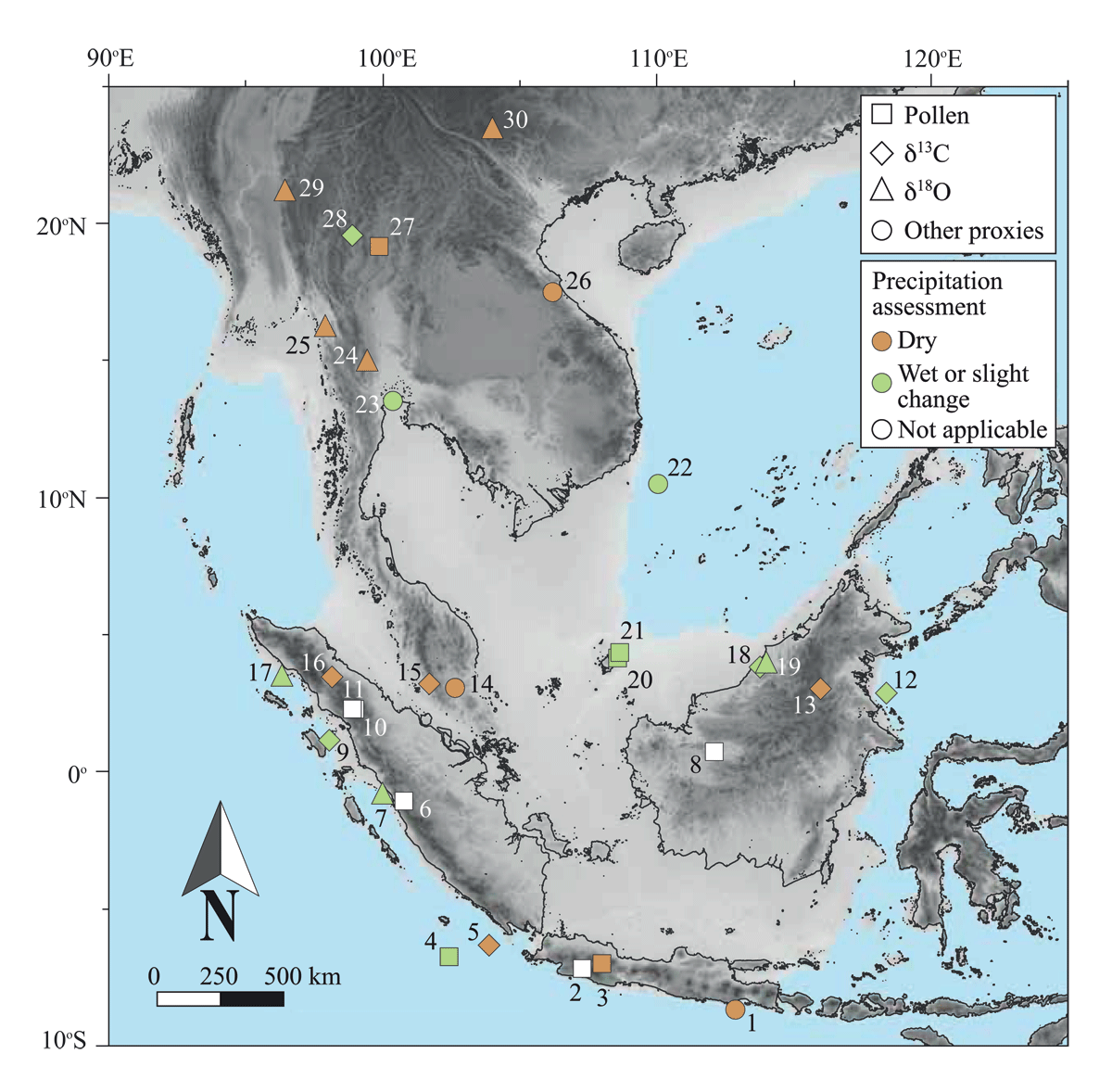
Figure 10
Compilation of the results obtained from the lower central plain of Thailand and the previous studies, indicate a comparable precipitation amount between the LGM and the present. See Table 3 for detail of each site.
Synthesizing our results with existing paleo-records from Mainland Southeast Asia (MSEA) and Sundaland during the LGM (Table 3 and Figure 10) reveals a spatially inconsistent but coherent rainfall patterns across the region. Drier conditions during the LGM were inferred from δ18O data in speleothems from Padamya Gu Cave (#25), Lin Noe Twin Cave (#29) in Myanmar, and an unnamed cave (#30) (Liu et al. 2020), as well as Mg/Ca and δ13C data from speleothems in Hoa Huong Cave, Vietnam (#26; Patterson et al. 2023) (Figure 10). However, the extent of the precipitation decrease remains uncertain, as reconstructions relied on comparisons of δ18O values from the LGM with recent values from speleothems in Hin Tum Cave (#24; Liu et al. 2020) and Phabaung Cave, which is separated by the Thanon Thong Chai Range. This mountain range might contribute to the depletion in δ18O observed in the speleothem records from Hin Tum Cave (#24; Liu et al. 2020).
Reconstructed LGM climatic conditions in northern Thailand were inconsistent between Kwan Phayao (#27; Penny & Kealhofer 2005) and Tham Rod Rockshelter (#28; Suraprasit et al. 2021) (Figure 10). Pollen records from Kwan Phayao indicate drier conditions (#27; Penny & Kealhofer 2005), while δ13C data from human and faunal tooth enamel at Tham Rod Rockshelter suggest a mixed tropical forest/grassland environment similar to the present climate (#28; Suraprasit et al. 2021). This inconsistency may reflect the limitations of pollen records in accurately capturing precipitation changes. Pollen records, while valuable, can be influenced by a variety of factors and may not always provide a complete picture of past climates. For instance, the pollen record from Lake Pa Kho, approximately 400 km northeast of Kwan Phayao, indicates a decrease in temperature but infers lower precipitation during the LGM, associating cooler conditions with dryness (Penny 2001). In contrast, proxies at Tham Rod Rockshelter (#28) point to the wetter conditions, supported by faunal remains (Wattanapituksakul 2006) and δ18O data from freshwater bivalves (Marwick & Gagan 2011).
Evidence for the LGM wet conditions includes high freshwater input to the Mekong River mouth (#22; Colin et al. 2010), western Sumatra (#7, #9, #17; Mohtadi et al. 2014; #4, van der Kaars et al. 2010), and southern Java (#1; Mohtadi et al. 2011) (Figure 10). These conditions were further corroborated by lowland rainforest and lower montane rainforest pollen assemblages in marine cores SO18302 (#20) and SO18300 (#21) near Natuna Island (Wang et al. 2009) (Figure 10). In contrast, a low sedimentation rate of organic-rich material in the Tasek Bera basin (#14; Wüst & Bustin 2004) in Peninsular Malaysia is linked to LGM sea-level regression and lower precipitation than present levels (Figure 10).
Pollen records from Pee Bullok Swamp (#10; Maloney & McCormac 1996), Pee Sim Sim (#11; Maloney 1980), di Atas Lake (#6; Newsome & Flenley 1988) in Sumatra, Situ Bayongbong Swamp (#2; Stuijts et al. 1988) in Java, and Sentarum Lake (#8; Anshari et al. 2001) in Borneo indicate cold conditions, though precipitation changes remain ambiguous (Figure 10). δ18O data from a cave in Gunung Buda National Park (#19; Partin et al. 2007) suggest slight changes in rainfall in Borneo between the LGM and modern times (Figure 10).
Meanwhile, the persistence of C3-dominant vegetation in Borneo, inferred from δ13C data in bat guano at Niah Cave (#18; Wurster et al. 2010) and δ13Cwax in marine core BJ8-03-91GGC (#12; Dubois et al. 2014), indicates wet conditions (Figure 10). Interestingly, δ13C data from Liang Mbelen Cave, Sumatra (#16; McCarthy et al. 2022), Batu Cave, Malay Peninsula (#15; Wurster et al. 2019), and Saleh Cave, Borneo (#13; Wurster et al. 2019), all located at similar latitudes, demonstrate C4-dominant vegetation, implying the LGM drier conditions (Figure 10). Pollen records from Bandung Basin (#3; van der Kaars & Dam 1995) further suggest low rainfall intensity during the LGM (Figure 10).
Although the LGM climate reconstruction in the northern part of MSEA is uncertain, dry conditions in Lin Noe Twin Cave (#29) in Myanmar and an unnamed cave (#30) in south China suggest that the mean position of the Intertropical Convergence Zone (ITCZ) possibly did not move north of 20°N in Sundaland, consistent with paleo-data and model comparisons by Chabangborn et al. (2014) and Liu et al. (2020) (Figure 10). Our results, along with other records from the emerged Sunda Shelf, indicate insignificant changes or increased precipitation between the LGM and present (Wang et al. 2009; Partin et al. 2007; Wurster et al. 2010). These findings suggest that Sundaland likely experienced a tropical wet-dry or savanna climate (Aw), similar to the present climate of much of MSEA as classified by Köppen (Peel et al. 2007). The LGM intense rainfall can be explained by the LMDz atmospheric general circulation model, simulating the additional precipitation contributed to the exposure of the Sunda shelf through the increase in the land-sea thermal contrast and moisture convection (Sarr et al. 2019). This, along with the flat palaeogeography of Sundaland, allowed humidity to be transported not only from the Indian Ocean but also from the South China Sea through the Pacific Trade winds during the summer. In contrast, anticyclonic flow or divergence possibly developed over the exposed Sunda shelf, causing lower precipitation during winter. These factors indicate intense seasonality differences in Sundaland, which may have continued toward the late MIS3 (Yamoah et al. 2021).
6. Conclusions
The analysis of K/Ti ratios, mean grain size, and sedimentary components from the lower central plain of Thailand between the Chao Phraya and Tha Chin Rivers, has provided valuable insights into the climatic fluctuations during the Last Glacial Maximum (LGM). The findings suggest a pattern of increased fluvial runoff and precipitation between 26.5 and 24.6 cal ka BP, followed by a brief period of reduced discharge around 24.6–24.1 cal ka BP, coinciding with Heinrich event 2. Subsequently, a gradual decline in runoff occurred until 23 cal ka BP, with another significant increase in precipitation from 23–22.8 cal ka BP, before an abrupt shift to drier conditions post-22.8 cal ka BP. These results indicate variability in the LGM climate, contrasting with the generally accepted notion of persistent cool and dry conditions due to a weakened summer monsoon. Our results align with paleo-records from Sundaland, showing substantial regional differences in precipitation patterns. Specifically, the wetter conditions during the LGM in parts of Sundaland were corroborated by increased freshwater input and pollen records indicating lowland rainforest prevalence. However, the climatic reconstructions also reveal inconsistencies, particularly in northern Mainland Southeast Asia, where evidence from speleothems and pollen records show both drier and wetter conditions. This discrepancy highlights the complexity of regional climate dynamics and suggests that the Intertropical Convergence Zone (ITCZ) did not shift significantly north of 20°N during the LGM. The synthesis of new and existing paleo-data suggests that the Sundaland climate during the LGM was similar to the present tropical wet-dry or savanna climate, with significant seasonal differences. The decreased rainfall in western Sundaland aligns with a weaker summer monsoon, potentially offset by increased land-sea thermal contrast due to the exposed Sunda shelf. This complex interplay of factors underscores the intense seasonality and regional climatic variations during the LGM, extending towards the late Marine Isotope Stage 3.
Additional File
The additional file for this article can be found as follows:
Supplementary 1
The concentrations of selected geochemical elements, including Fe, K, Cl, Ti, Ca, Ba, Br, Zr, Rb, Sr, and Zn, derived from the sedimentary sequence of the Lower Central Plain, Thailand. DOI: https://doi.org/10.5334/oq.154.s1
Competing Interests
The authors have no competing interests to declare.