
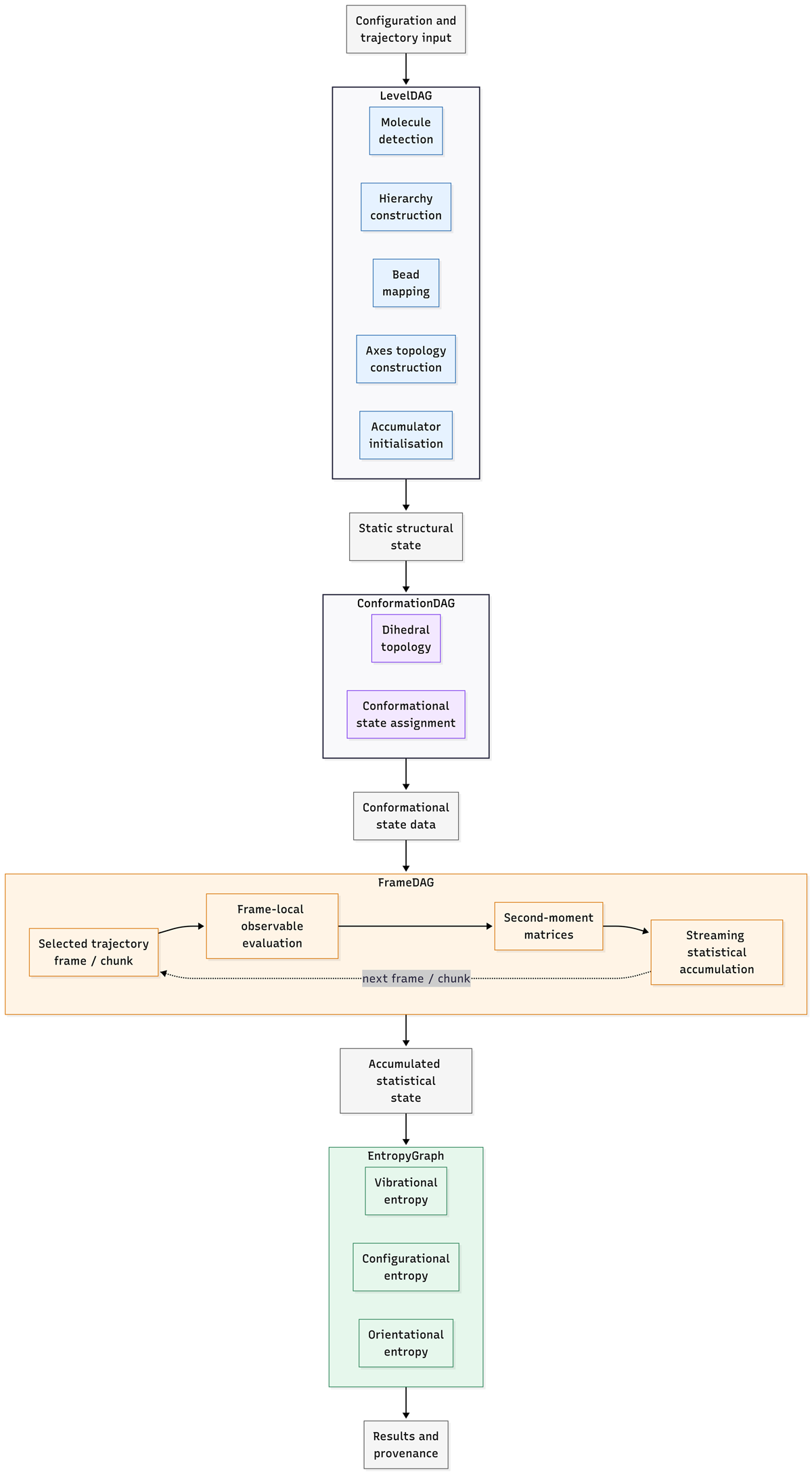
Figure 1
Overview of the CodeEntropy workflow showing static setup, conformational state construction, frame-level statistical accumulation, and final entropy evaluation.
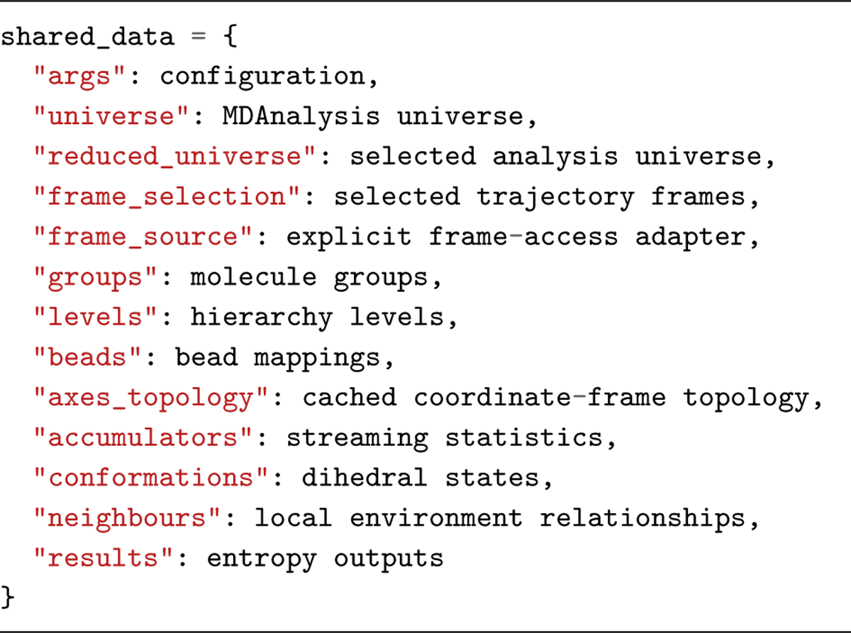
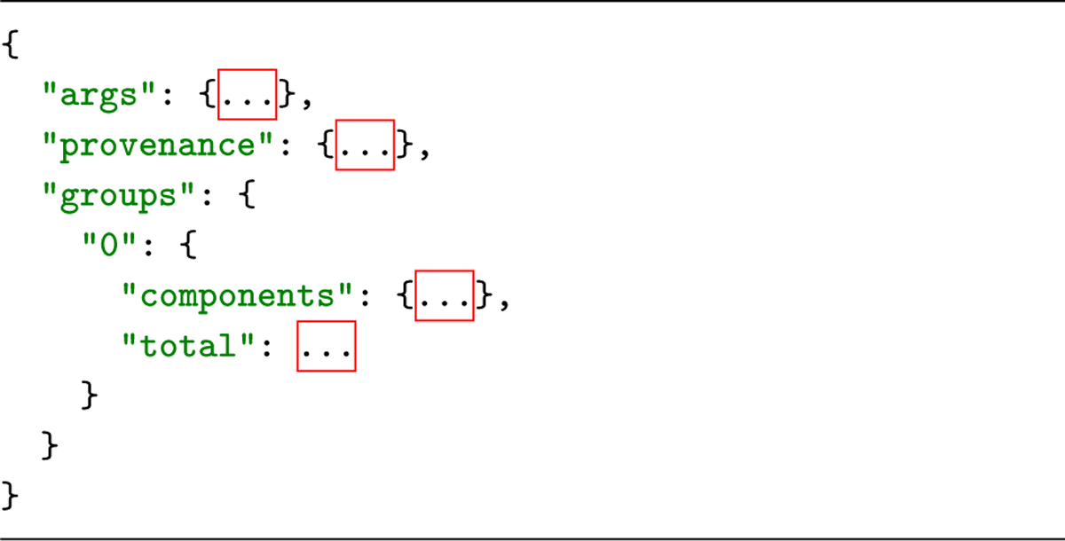
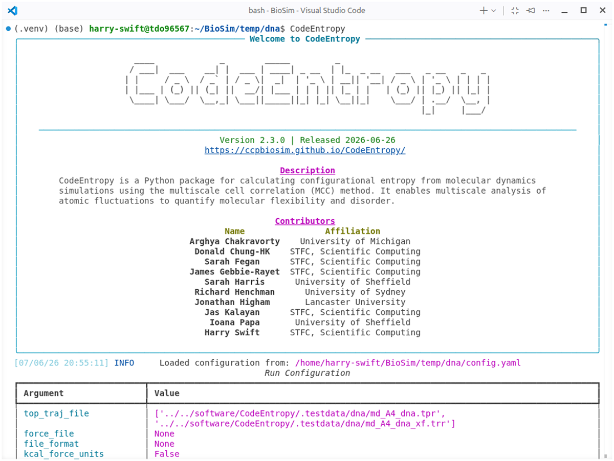
Figure 2
Command-line interface splash screen displayed during program initialisation, showing software identity and execution context.
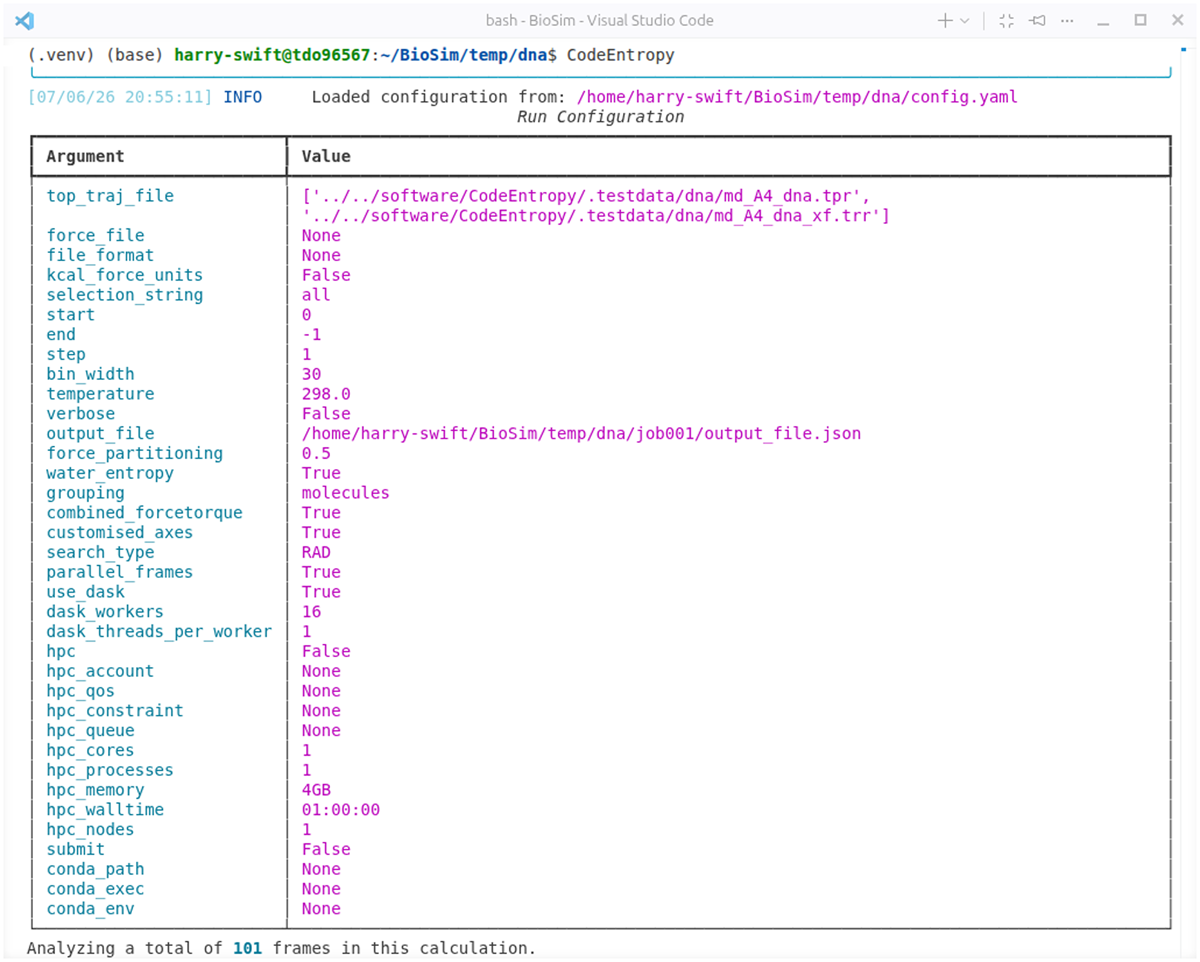
Figure 3
Example runtime configuration loaded from a YAML file, illustrating user-defined analysis parameters and workflow options.
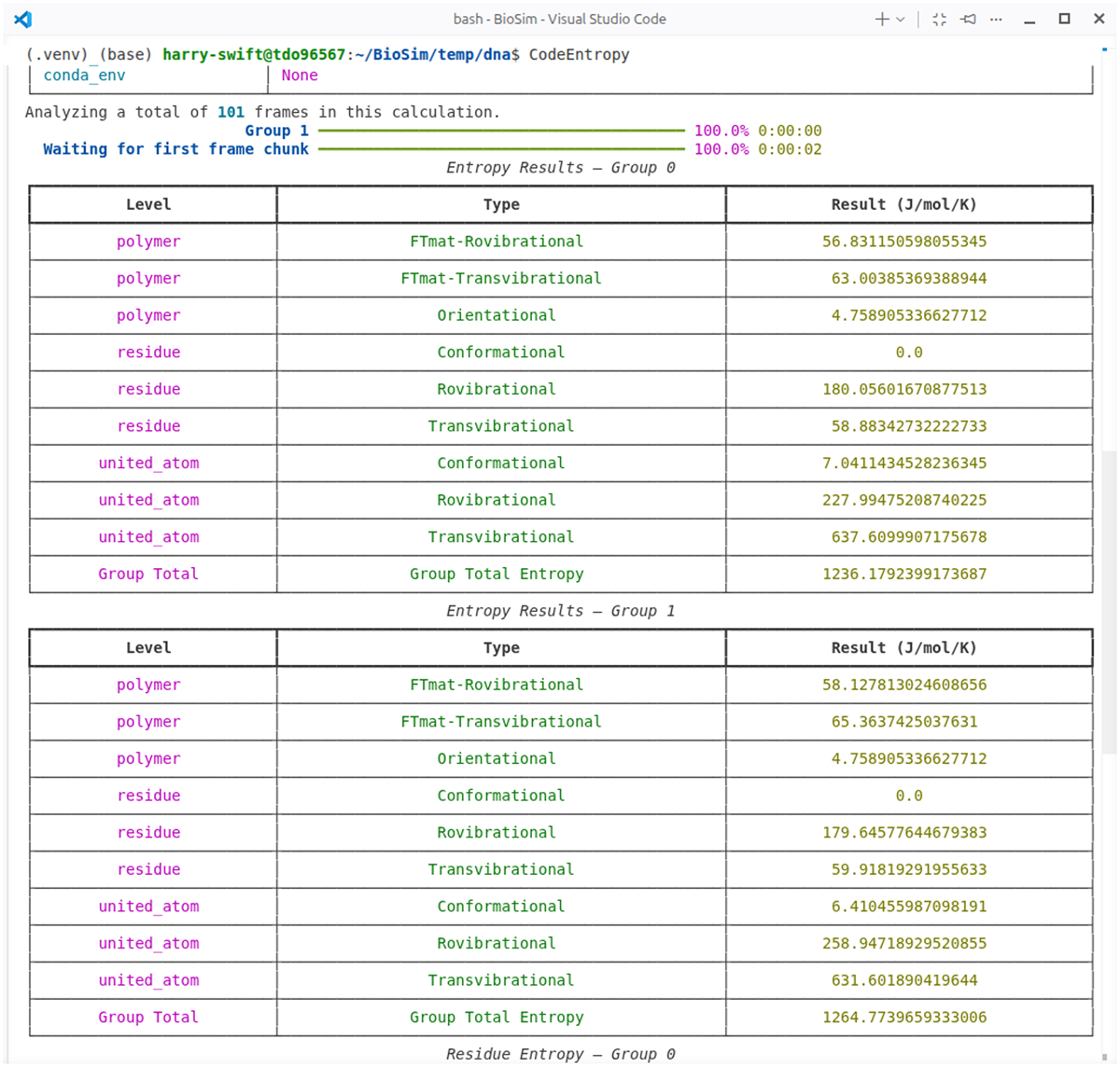
Figure 4
Terminal output showing aggregated entropy results, including total and component contributions computed from the accumulated statistical model.
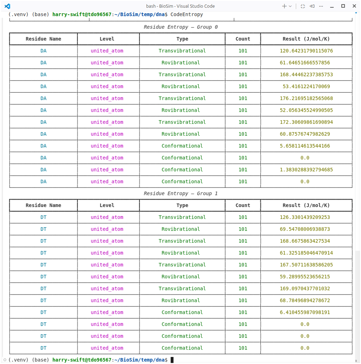
Figure 5
Residue-level entropy decomposition presented as tabulated terminal output, illustrating how total entropy contributions are distributed across molecular components.
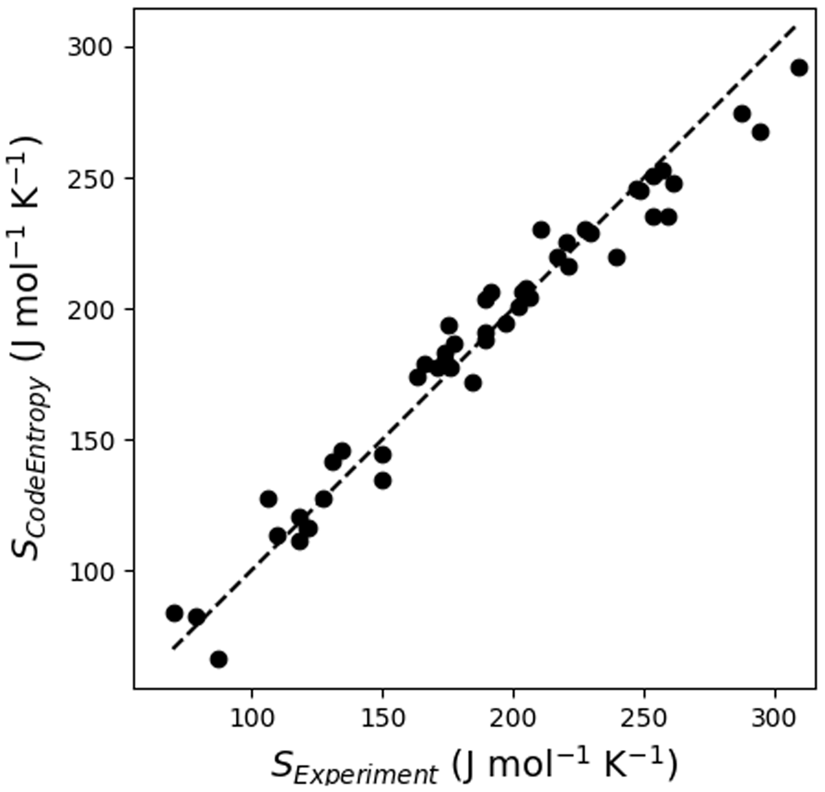
Figure 6
Entropy of 49 liquids from CodeEntropy versus experiment. The dashed line represents perfect agreement. Error bars are negligible.
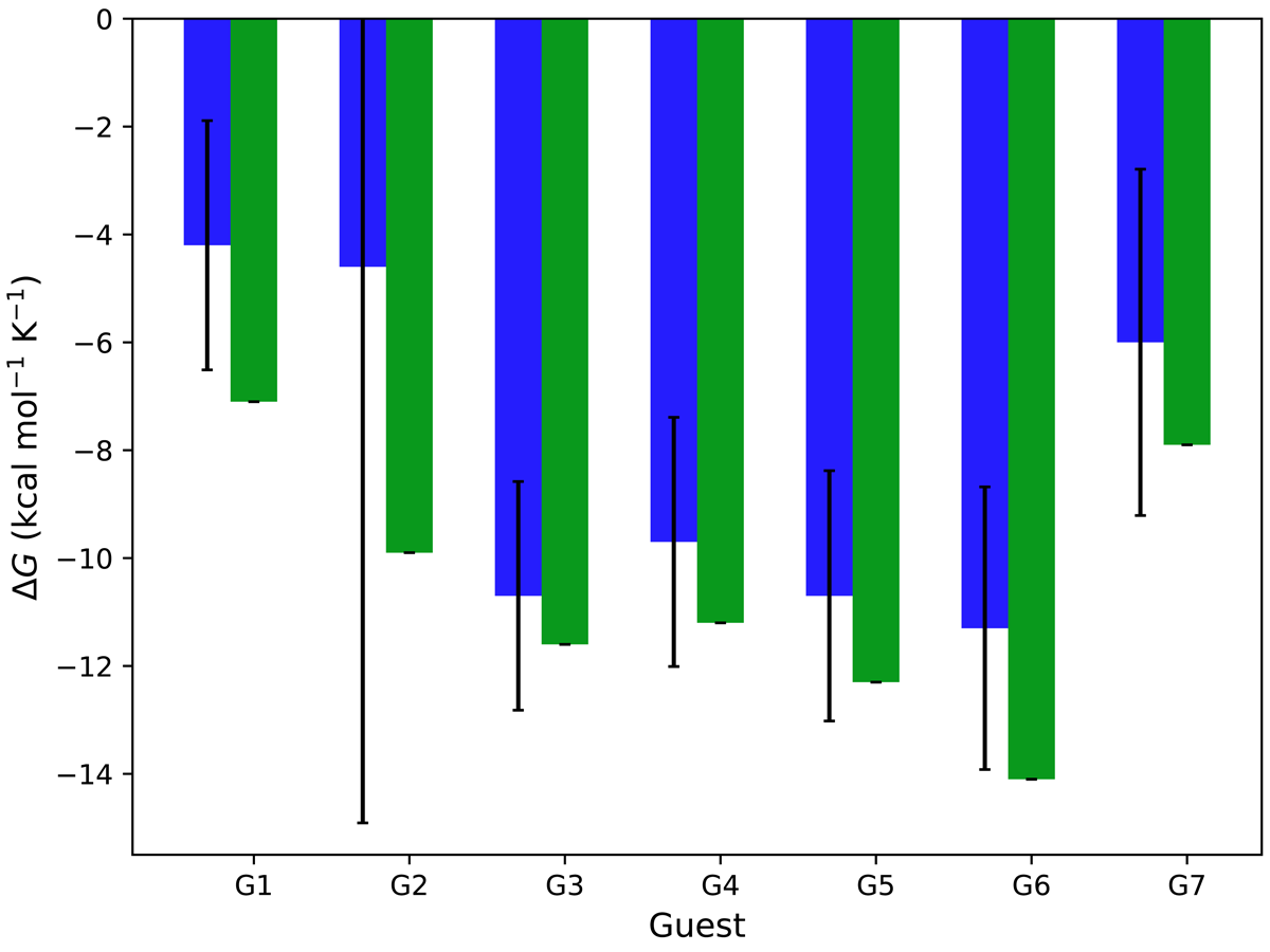
Figure 7
CodeEntropy binding Gibbs energies (blue) versus experiment (green) for the host-guest systems in the SAMPL8 challenge.