KernelPopper: A Scikit-Learn Compatible Package That Calculates Feature Weights From Trained Kernel Ridge Regression Models

Introduction

Linear least squares regression is a supervised learning method for modelling the relationship between features and a target variable. It has been modified, generalized and extended, and implemented in many programming languages, including the widely used Python library scikit-learn (1). While deep learning can surpass simpler methods on complex datasets, the least squares model family has several practical advantages: the approach is parsimonious, and the learned feature weights provide insights into the importance of features that govern the model’s performance, thereby suggesting hypotheses for the causal effects that determine the target variable. Linear models and least squares regression, thus, remain popular approaches for data analysis.

Given some data (X, an n × l matrix containing n feature vectors x₁, x₂, …, x_n, each of length l), and corresponding values of a target variable (n-length vector y), the aim of least squares regression (2, 3) is to find a set of coefficients (l-length vector w) that determine a linear relationship between features and an output variable with the least deviation from the desired target values. These coefficients, the components of the vector w, are termed feature weights, with each one corresponding to one of the l features in the input matrix. These components are also referred to as primal coefficients.

The feature weights can be found by linear algebra,

Given a new data point (feature vector $\widehat{x}$), the target variable can be predicted from the feature weights,

where c is a constant known as the bias or intercept.

Several modifications to least squares have been introduced to increase the robustness to noise and reduce the tendency to overfit. The LASSO and ridge methods incorporate L1- and L2-norm regularization, respectively; the ElasticNet method combines both. LASSO encourages sparse coefficients, whereas ridge regression encourages a smaller sum of the absolute values of coefficients (4).

The ridge regression model (2) learns from a matrix of features belonging to a set of training samples, X, and the target variable for each training sample, y, learning the feature weights,

where I is the identity matrix and λ is a parameter defining the strength of L2-norm regularization.

The scikit-learn library implements Kernel Ridge Regression (KRR) (5). This combines ridge regression with the “kernel trick”, which is a way to reframe problems that allows non-linear relationships to be learnt using linear algebra. It is performed by learning dual coefficients, α (n-length vector),

K is known as the kernel matrix, which is defined by the (i, j)^th entry being the result of a given kernel function, k(·), on the original feature vectors x_i and x_j (6). The kernel function can be any function that produces a real number that adheres to certain conditions (a Mercer kernel). The kernel matrix can be viewed as a matrix of the inner product of sample pairs in the new feature space, for which the features are determined by the kernel function (6),

where ɸ(…) is the mapping of a given original feature vector to a new, typically higher-dimensional, feature vector in the new feature space. For example,

is the linear kernel function that implicitly defines the mapping from input space to feature space. In this case, ɸ(x) = x. An example of a more complicated kernel is the radial basis function (RBF) kernel,

which defines ɸ(x) as an infinite-dimensional feature vector. These new features (known as implicit features) do not need to be enumerated as only the kernel matrix is required for training and inference. This means that the model training process remains efficient when the dimension in feature space increases (Figure 1).

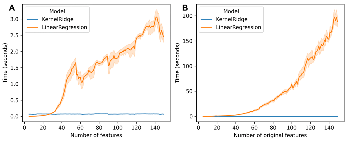
Figure 1

Within this framework, the target variable for a new sample ($\widehat{x}$) can be predicted from the dual coefficients, α,

As the kernel function is equivalent to an inner product, the predicted target can be expressed in this form,

where the feature weights can be calculated from the dual coefficients (7, 8),

This sum of l-length vectors is itself an l-length vector, meaning that for some choices of kernel, such as for the RBF kernel that induces an infinite-dimensional feature vector, the input space vectors cannot be explicitly mapped to their feature space representation.

KRR with polynomial kernels are used across domains, with recent examples including the prediction of crop yields (10), economic forecasting (11), clinical research (12), and rainfall forecasting (13). While feature weights calculated from dual coefficients have been used previously to identify potential learned relationships from training data (14), this has been performed with non-reusable code within other projects. The Himalaya package provides this functionality, but only for linear kernels (15). Here, we introduce KernelPopper, which can calculate feature weights for KRR problems solved using polynomial kernels of the second and third degree.

This tool was produced for our ongoing work focusing on molecular dynamics (MD) simulations of liquid–liquid phase separation (LLPS) (16). We used MD to produce simulations of proteins and miRNA molecules that capture the process of LLPS, in which liquid droplets form within the bulk liquid and partition the system. We are extending this research by training machine learning models on the simulations to predict rates of intermolecular contact and are interested in whether the weights learned by the models conform to known LLPS patterns or might indicate new patterns. The data is presented to the models in one-hot encoded sequences of amino acid and so it contains hundreds of features, which has necessitated the development of KernelPopper. Given the potential use of this tool for other projects, we have made this tool available as a Python package.

(1) Implementation and Architecture

We have taken a functional approach to implementing KernelPopper; the pop.py file in the source code contains two separate functions, get_quadratic_weights and get_cubic_weights, for use on trained models with polynomial kernels of degrees two and three, respectively. Each function accepts a trained KernelRidge model and returns feature weights in a dictionary object along with new predictions, as well as the samples mapped into feature space for testing and further analysis.

In this work, we focus on the polynomial kernel function as defined in scikit-learn (1):

where x and z are the input feature vectors, c is a constant additive term, 𝛾 is a constant scaling factor, and d is the degree of the polynomial. To find the implicitly defined features of ɸ(x) induced by this kernel, we must make the terms of the inner product explicit. We first expand the polynomial function and then factor it into vectors of features of x and z, thereby defining the functions ɸ(x) and ɸ(z).

The expansion depends on the degree and on the dimension of x and z. For example, if the degree d = 2 and the feature vectors are one-dimensional, i.e., contain one feature each, the kernel function of x and z is equivalent to the scalar product of the following new feature vectors, i.e., the scalar product of ɸ(x) and ɸ(z), $\left[c, x_1\sqrt{2c\gamma }, \gamma x_1^2\right] \cdot \left[c, z_1\sqrt{2c\gamma }, \gamma z_1^2\right]$ (6, 17, 18).

This kernel thus gives rise to the following new features: the constant, c; $\sqrt{2c\gamma }$ multiplied by the feature; the scaling hyperparameter γ multiplied by the square of the feature. For this quadratic polynomial, each additional original feature, f, in the input matrix adds two implicitly defined features, $f\sqrt{2c\gamma }$ and γf², as well as combined terms with each other feature, $\gamma f_1{f}_2\sqrt{2}$ (17, 18). The get_quadratic_weights function computes all these implicit features that are used to drive regression in the case of a quadratic kernel function, but which typically remain hidden during the training process.

The get_cubic_weights function computes the feature weights for the case where the function is of degree d = 3. Along with the constant $\sqrt{c^3}$, each input feature introduces three features, implicitly defined by the kernel: $f^3\sqrt{{\gamma }^3}$; $\gamma f^2\sqrt{3c}$; $cf\sqrt{3\gamma }$. Each pair of input features also introduces three implicit features: $\gamma f_1{f}_2\sqrt{6c}$; $f_1^2{f}_2\sqrt{3{\gamma }^3}$; $f_1{f}_2^2\sqrt{3{\gamma }^3}$. Finally, each combination of three input features results in an implicit feature of the form $f_1{f}_2{f}_3\sqrt{6{\gamma }^3}$.

The KernelPopper tool is implemented as a Python package, which can either be installed through PyPI using the command python3-m pip install kernelpopper or through the source code at https://github.com/ruth-veevers/kernelpopper and then incorporated into the user’s own Python code or notebooks. Two main functions calculate the feature weights, and the user selects the appropriate version: get_quadratic_weights if the fit model uses a polynomial kernel of the second degree; get_cubic_weights if the model’s polynomial kernel is of the third degree. Figure 2 shows an example of KernelPopper working to retrieve meaningful feature weights from a model trained on synthetic data.

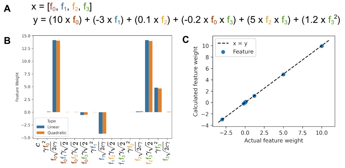
Figure 2

(2) Availability

(3) Reuse potential

The software will be of interest to researchers who use scikit-learn’s KernelRidge model to perform regression with polynomials up to a degree of three. We anticipate a typical re-use scenario in which a researcher has trained a KernelRidge model for a regression problem from their domain and wants to evaluate what that trained model has learned and what features are driving the predictions. They install the package through PyPI using the command “python3-m pip install kernelpopper”. If their model uses a polynomial kernel with degree two, they import the get_quadratic_weights function. They call this function, passing their trained model as the first argument, followed by an optional list of strings that describe each input feature. The function returns three objects. The first is a dictionary where the keys are descriptions of the implicit features as combinations of the input features; as the researcher passed in a list of their input feature names, their names are used to populate this dictionary. Without passing in the optional name list, dummy feature names would be used, such as “f0”, “f1”, and so on. The values of the dictionary are the feature weights that correspond to each implicit feature. The user can then analyze the magnitude and sign of the feature weights to develop hypotheses for the underlying relationships in the data. The get_quadratic_weights function also returns predictions for the original regression problem calculated from the feature weights, which should be the same as the predictions returned by the trained model; the user can compare these to ensure that the function has worked as expected. The final returned object is the full list of samples mapped to feature space, which the researcher may want to use in their plotting or further analysis. A Jupyter notebook linked from the GitHub repository shows an example of this use case.

While it is possible to generalize the presented functions to higher orders, we limited our implementation to polynomial kernels of the second and third degree for computational and application reasons: higher order polynomials scale increasingly poorly with data size, and the number of feature combinations produced would make it increasingly difficult to interpret weights. Contributions are welcomed via GitHub pull requests. Support requests will be addressed using Github’s Issues functionality.