
(1) Overview
Introduction
The Distance-based Generalized Sensitivity Analysis (DGSA) methodology [1] was developed to quantify both single parameter sensitivities and complex parameter interactions, as in many engineering and geoscience applications, combinations of model parameters can have a significant impact on model responses [2]. In addition to computing and ranking single parameter sensitivity, DGSA also provides the sensitivity of one parameter conditioned to setting another parameter to different ranges. This allows for capturing asymmetric parameter interactions, where the sensitivity of parameter A given parameter B could differ from the sensitivity of parameter B given parameter A in a complex model. DGSA makes no assumptions on the parameter distribution, nor is there a need to interpolate model responses. It can be used with discrete or continuous variables and multidimensional responses (time-varying, multiple responses, etc.). It belongs to the global sensitivity analysis techniques [1].
DGSA clusters model responses into distinct groups using the K-medoids clustering algorithm. Then, for each parameter, the cumulative distribution functions (CDFs) are compared between all clusters. If clusters have similar CDF distributions, it implies that the parameter (on its own) has little impact on the model responses used for clustering and is therefore considered as insensitive. On the other hand, differences among cluster CDF distributions indicate a significant influence on model responses, and hence, high parameter sensitivity. The same approach can be extended to compute conditional parameter sensitivity. In addition to clustering based on model responses, each parameter is binned into distinct groups. By comparing CDF distributions among clusters and bins, one can quantify the combined sensitivity of one parameter conditioned to another parameter. DGSA offers two methods for standardizing the sensitivity measure. The first method computes the observed L1-norm distances between CDFs and normalizes them with a bootstrapped L1-norm distance at the user-specified quantile (L1-norm method). The other method calculates the quantiles of the observed L1-norm distances in all bootstrapped L1-norm distances (achieved significance level (ASL) method, from 0 to 100%). These two methods produce highly comparable and consistent sensitivity rankings. For a detailed explanation of the DGSA methodology, we refer readers to [1] and [2].
Two MATLAB versions of DGSA exist [3, 4]. There is also a ‘light’ Python version [5] that implements only single parameter sensitivity analysis. This new Python version includes all the key functionalities from the MATLAB versions with the following improvements: i) Python vectorization reduces looping and improves speed, ii) functions for sensitivity computation are combined and reorganized to make the code cleaner, iii) plotting is more customizable, iv) a perceptually uniform colormap is used to avoid biased interpretations of sensitivity results, and v) extensive code comments are added to facilitate easy understanding. Our goal is to provide a new Python DGSA tool that integrates all functionalities, making it more accessible than a MATLAB implementation.
Implementation and architecture
DGSA was implemented as Python functions that are grouped into two folders: computation and visualization. The computation folder contains functions for computing K-medoids clustering, as well as single and conditional parameter sensitivities. The visualization folder includes functions for generating Pareto plots for single parameter sensitivity, heatmaps for conditional parameter sensitivity, CDF curves by clusters and bins, and multidimensional scaling of model response clusters (Figure 1). Some functions contain subfunctions allowing for complex computation to be broken into simpler and easier-to-understand pieces. All functions and subfunctions include detailed docstrings explaining the meaning and format of input and output data, as well as comments explaining each computation step. For functions involving random processes, including initialization for K-medoids clustering and bootstrap sampling for sensitivity calculation, a random seed is needed to ensure reproducibility.
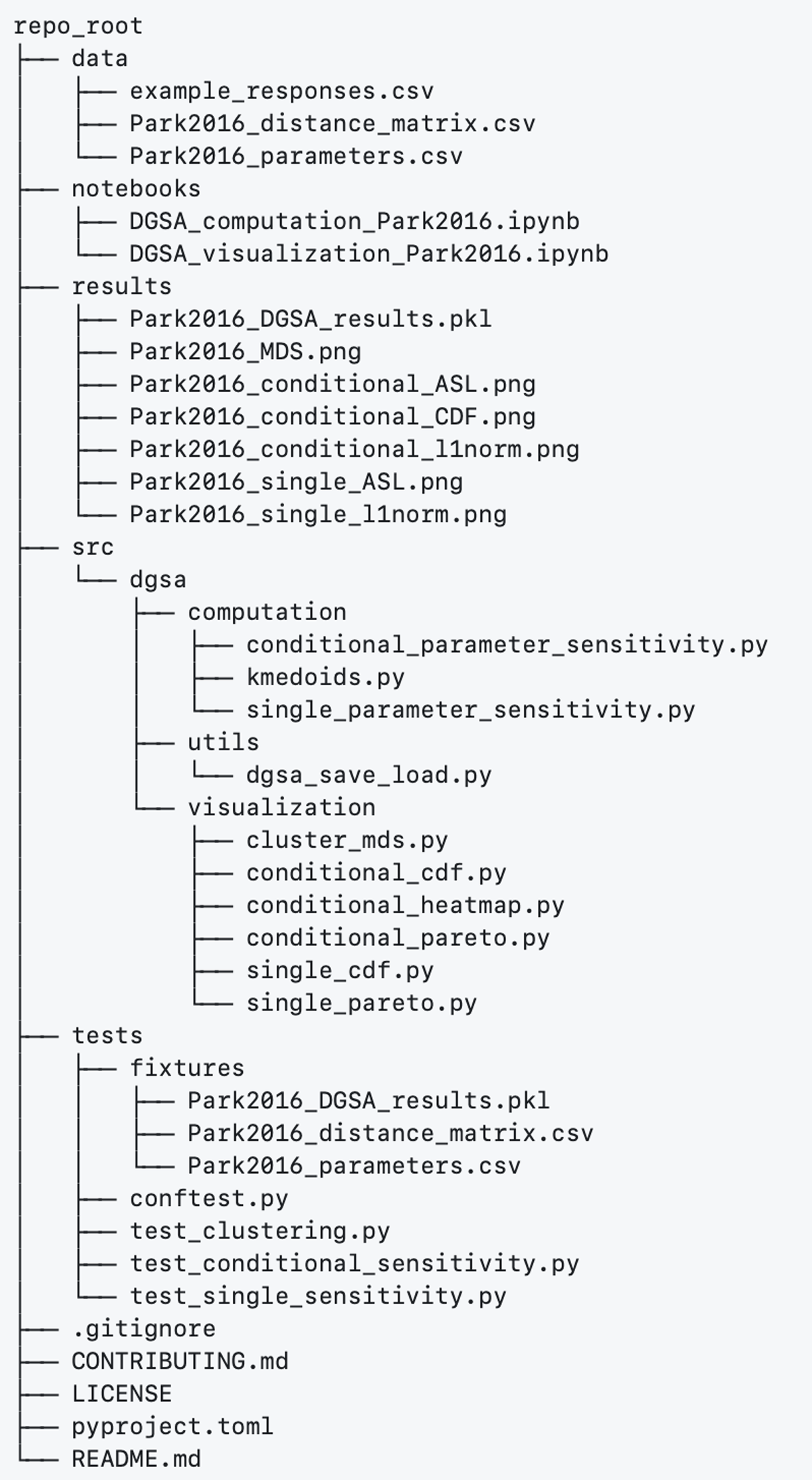
Figure 1
GitHub repository structure of the Python DGSA package. Data folder contains example dataset, notebooks folder provides two Jupyter notebooks to illustrate usage, example results are saved in the results folder, all source codes are included in the src folder, and the tests folder supports pytest functionality. Single files including CONTRIBUTING.md, LICENSE, pyproject.toml, and README.md provide information on collaboration, license, installation, and general instructions.
To perform DGSA, users need to install the package following the instructions in the README.md, prepare model parameter and response samples as CSV files, and then directly call functions to compute sensitivities and generate plots. To illustrate how to use the code, an example dataset from Park et al.’s work [6] and two Jupyter notebooks are provided (Figure 1). The computation notebook demonstrates how to compute single and conditional parameter sensitivities and save the results. The visualization notebook shows how to generate various plots from the saved sensitivity results (Figure 2). Users can follow the same workflow for their own analysis.
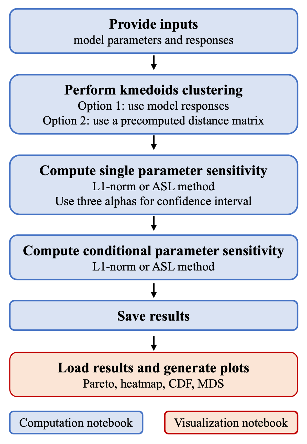
Figure 2
DGSA workflow implemented in the computation and visualization Jupyter notebooks. These two notebooks use an example dataset to illustrate the procedure of performing DGSA.
The computational cost of the DGSA scales primarily with the number of model runs (n_samples), the number of parameters (n_parameters), and the number of bootstrap iterations (n_draws). For the example dataset (n_samples = 1,000; n_parameters = 15; n_draws = 3,000), single and conditional sensitivity analyses complete in under 40 seconds and 4 minutes on a standard laptop, respectively. Python vectorization (NumPy) is used throughout to minimize looping. Users working with large datasets (e.g., n_samples > 10,000, n_parameters > 50) may consider reducing bootstrap iterations or using high-performance computing to manage runtime.
Quality control
To ensure the accuracy of analysis, the Python DGSA has been validated against the original MATLAB version [3] using the same dataset from Park et al.’s work [6]. Based on flow simulations on a Libya oil field, the example dataset contains a total of 15 continuous and discrete model parameters and 1,000 water production predictions as model responses. Figure 3 shows the comparison between Python and MATLAB single parameter sensitivity results using the L1-norm method. Figure 4 compares the conditional sensitivity results of the Python version with those of the MATLAB version. In this case, the ASL method was used. To quantify how similar the results are, the concordance correlation coefficient (CCC) was calculated, which measures similarity based on both correlation and bias. The CCC scores are 0.9997 and 0.9875 for single sensitivity (Figure 3) and conditional sensitivity (Figure 4), respectively. With the CCC scores very close to 1, it demonstrates that the Python version produces similar sensitivity measures to the MATLAB version. The small differences come from the random nature of bootstrapping in both L1-norm and ASL methods and the lack of random seed control in the MATLAB version. Also, note that when two parameters have similar sensitivity measures or extreme ASL values (e.g., 99.9+), their ranking may differ between versions and methods, again due to the random sampling. These comparisons demonstrate that the Python DGSA performs sensitivity analyses with accuracy comparable to the MATLAB version. For users to check if the package is working properly, simply run the workflow in the notebooks using the example dataset, and compare with the example results (Figures 1 and 2). There is also an option to run a pytest protocol to verify package accuracy.
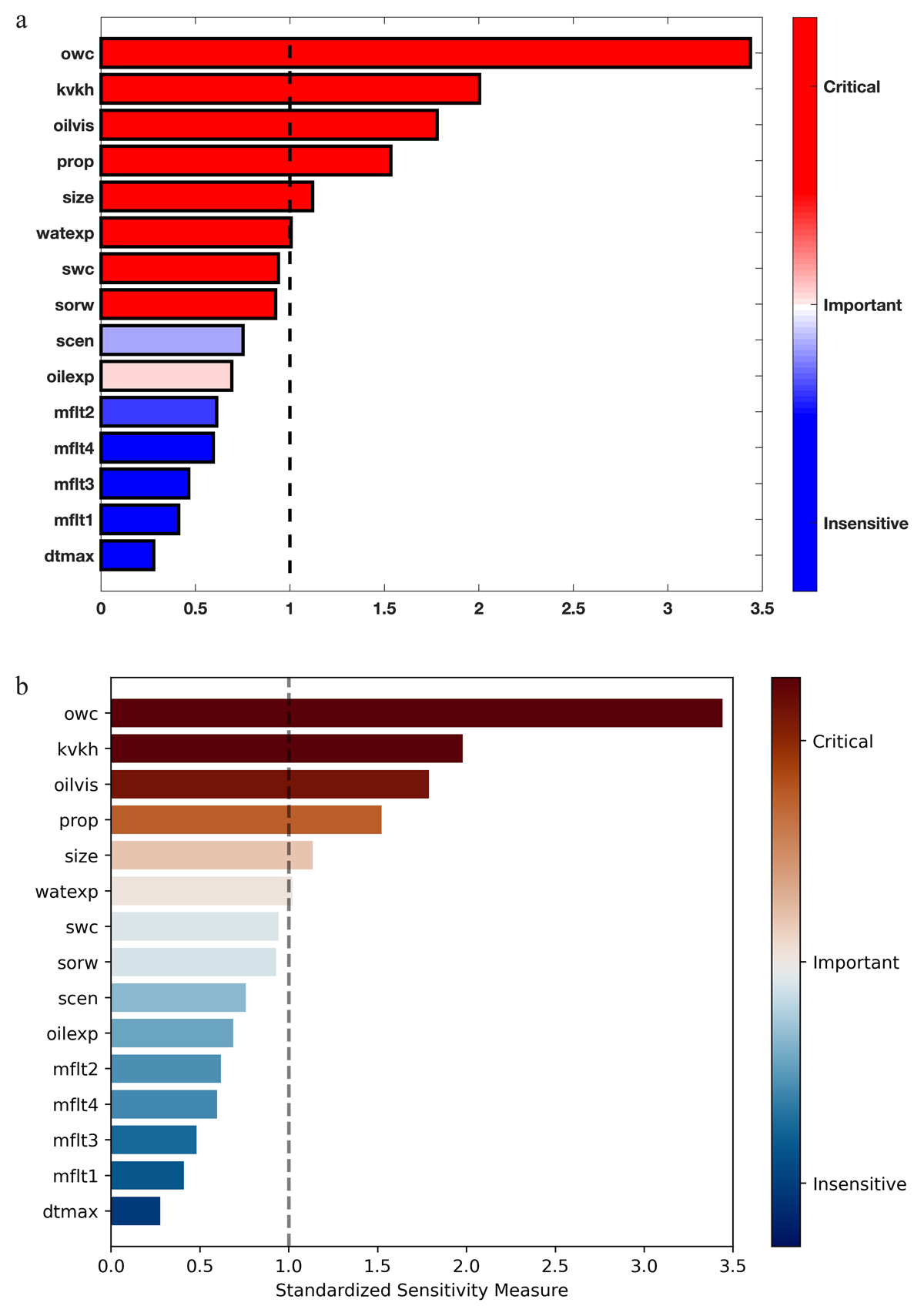
Figure 3
Comparison of single parameter sensitivity using the L1-norm method between the MATLAB (top) and Python (bottom) versions. The CCC for this comparison is 0.9997, which demonstrates that the Python version produces similar sensitivity measures to the MATLAB version.
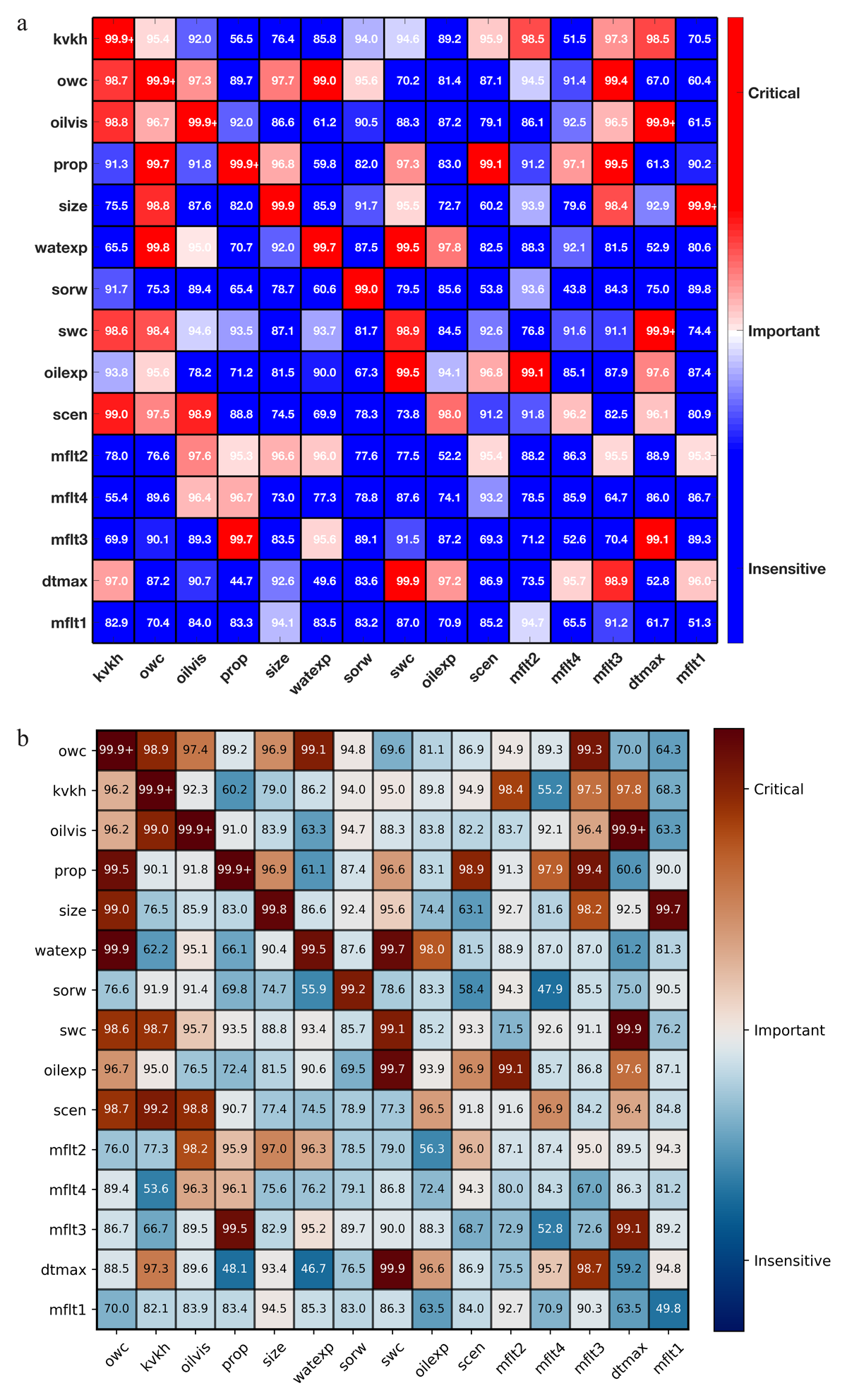
Figure 4
Comparison of conditional parameter sensitivity using the ASL method between the MATLAB (top) and Python (bottom) versions. The CCC for this comparison is 0.9875, which demonstrates that the Python version produces similar sensitivity measures to the MATLAB version.
(2) Availability
Operating system
Windows, macOS and Linux.
Programming language
Python version 3.6 or above.
Additional system requirements
None.
Dependencies
Python packages: numpy, pandas, matplotlib, scipy, sklearn, cmcrameri.
List of contributors
Jihui Ding – Code development, manuscript writing, and revision
Céline Scheidt – Code review, manuscript writing, and review
Peng Li – Code review and manuscript review
David Zhen Yin – Manuscript writing and review
Jef Caers – Project mentor and manuscript review
Software location
Archive
Name: Zenodo
Persistent identifier: DOI: https://doi.org/10.5281/zenodo.20574779
Licence: MIT
Publisher: Jihui Ding
Version published: 1.0.0
Date published: 6/6/26
Code repository
Name: GitHub
Identifier: https://github.com/Stanford-Mineral-X/DGSA
Licence: MIT
Date published: 14/11/25
Language
English
(3) Reuse Potential
Geoscientific studies, such as geological modeling and physics simulation, often involve a large number of parameters with complex interactions [2]. The Python DGSA is well-suited for deciphering parameter sensitivities and their interactions, which is a key step in supporting decision-making and reducing model complexity. Because sensitivity analysis is a common practice in many fields, the Python DGSA can serve as a general sensitivity analysis tool. It accepts any modeling inputs and outputs, making it applicable beyond geoscience, to engineering, environmental modeling, climate science, and other fields involving complex numerical models. Example reuse scenarios include: (i) petroleum reservoir engineering, where DGSA can screen which petrophysical or geological parameters most influence production forecasts, supporting more targeted history matching; (ii) climate and hydrological modeling, where it identifies which forcing parameters dominate multi-variable outputs such as temperature, precipitation, or streamflow; and (iii) geotechnical and environmental risk assessment, where conditional sensitivity reveals parameter interactions governing slope stability or contaminant transport.
The Python DGSA package will be actively maintained and improved as an open-source tool on GitHub by the Mineral-X research group at Stanford University. External contribution is welcome for bug reports, feature requests, or any improvement suggestions. We will utilize GitHub Issues and Pull Requests as the primary channel for collaboration and package enhancement. The Python DGSA is modular, with computation and visualization functions that can be extended to incorporate new clustering methods, alternative sensitivity metrics, or customized visualizations. We welcome any contribution that makes the Python DGSA package a more useful tool for the research community.
Acknowledgements
We thank the members of the Stanford Mineral-X research group for supporting the development of this package, including KoBold Metal, Birdra, Ero Copper, Fleet Space Technologies, Ideon Technologies, Xcalibur, NorthIsle, and Edra Labs.