
(1) Overview
Introduction
Water resource managers and planners depend on observations and projections of hydroclimatic variables to understand the present and plan for the future. However, observations of past hydroclimatic conditions are often inadequate for use in planning because of deficiencies in their length, completeness, or spatial coverage [1], resulting in infrequent but consequential meteorological events (like droughts and floods) being underrepresented. Further, because weather is a stochastic process, the observations that are available represent a single possible trace from a range of plausible alternatives [2, 3]. These alternative realizations of weather which could have naturally resulted from the nonlinear, stochastic, dynamical, or interacting features of the climate system over different time scales—more generally referred to as the internal variability of the system [4, 5, 6]—are often not considered [7], exacerbating issues with data quantity and quality and reducing the investigable planning space. Accounting for the system’s hydroclimatic internal variability is therefore essential for water resources planning.
Under these conditions, water resource planners utilize ‘bottom-up’ methodologies [8, 9, 10] to focus more on what is of consequence to decision-making rather than what is most likely to happen, through exploratory modeling [11, 12] and stochastic sampling techniques [13, 14]. This approach generally involves exploring an ensemble of counterfactual states of the world through a statistical model that uses either truly exploratory ranges of parameters or extracted information from a combination of different downscaled projections and observations; these states of the world then shape the plausible stochastic realizations of weather that are treated as inputs to the hydrologic or land-surface models used in impact analyses [15, 16, 17]. Stochastic weather generators (SWGs) are statistical models that can simulate realistic, arbitrarily long sequences of regionally informed meteorological variables like precipitation and temperature and are thus popular tools for bottom-up sampling [1, 18, 19, 20]. In order to faithfully replicate the hydroclimatic statistics of a particular region, SWGs must account for both the spatial and temporal relationships of hydroclimatic observations. Most contemporary SWGs simulate at least precipitation and temperature since these two variables drive the types of outcomes that planning scenarios are typically quantitatively based on (e.g., water availability, irrigation water requirements, drought indices) [21]. But precipitation and temperature are nonlinearly related [22], so methods to sample them nonlinearly like copulas are necessary [23, 24, 25, 26, 27]. Further, weather is a complex spatial and temporal phenomenon and therefore the same mesoscale system might produce significantly different but correlated meteorology across the region of interest, especially over heterogeneous terrain [28, 29]. It follows that there is often a need for SWGs capable of nonlinear multivariate, multisite weather generation [20] to ensure spatial consistency.
Multivariate, multisite SWGs that utilize copulas to account for system nonlinearities represent the state of the art for weather generation [30, 31, 32, 33, 34, 35]. That said, the fitness of these existing multivariate, multisite SWGs largely depends on their ability to sample the relevant space sufficiently and replicate spatiotemporal correlations for historical observations or future projections. Therefore, SWGs built for regions influenced by weather regimes [30, 32, 34] will not be suitable in regions that are not influenced by the same large-scale phenomena. SWGs built for forecasting and downscaling from general circulation models (GCMs) [31] or that focus on a specific future projection [33] will miss exploring internal variability under the alternative states of the world inherent in the system. And SWGs built for weather events like droughts [35]—synthetically generating precipitation and temperature as an intermediate step—will prioritize the generation of hydroclimatic events that may simply not occur in other regions and therefore cannot be generalized. Additionally, existing weather generation tools miss more general applications by not being multisite [36, 37, 38, 39, 40] or by only being a downscaling product for GCMs [41, 42], and they largely do not contain sufficient (if any) validation tools or open-source software packages [43, 44]. Finally, while frameworks and software implementations for generating individual hydroclimatic variables with arbitrary marginal distributions and correlation structures exist [45, 46, 47, 48], they are limited by their ‘parent’ Gaussian processes in that only linear dependence in the Gaussian space can be captured, potentially missing the nonlinear conditional dependencies between these variables.
For these reasons, in this paper we introduce swxg, a Python library for generalized multivariate, multisite, copula-based stochastic weather generation that by design can also be integrated into exploratory modeling contexts. Our SWG is solely focused on replicating a region’s underlying spatiotemporal hydroclimatic correlations and statistics and is therefore applicable for regions that either have weather regimes or do not, for synthetically generating weather variables as an intermediate step or for their own sake, or for explorations of internal variability more broadly. swxg accomplishes this by first taking input observations of precipitation and temperature at one or more sites and performing a semiparametric fitting and generation of precipitation. It then conditionally generates temperature from a copula fit to historical precipitation and temperature data. Further, swxg formalizes a set of validation figures to both numerically and visually confirm its goodness of fit, a feature yet to be included in other generators. By generalizing stochastic weather generation in this way, swxg represents a novel, flexible bottom-up assessment tool for a wide range of use-cases.
Implementation and Architecture
swxg has been developed as a Python library containing data structures and classes necessary to stochastically generate weather from two statistical models—one for precipitation and one linking precipitation to temperature via copulas—trained on an input dataset of observations. A byproduct of this statistical interpretation is the associated fitness of each model for all hydroclimatic variables and sites, where each is assessed, analyzed, and presented to the user for them to be able to make their own determinations about whether the fitting process has performed adequately. It is designed for a streamlined workflow in which users interface solely with the SWXGModel() class, which handles formatting the input observations, statistically fitting marginal and joint distributions, validating the statistical fits, generating synthetic weather, and comparing the generated weather to the original observations. An outline of this workflow along with critical methods, arguments, and validation checks are included in Figure 1.
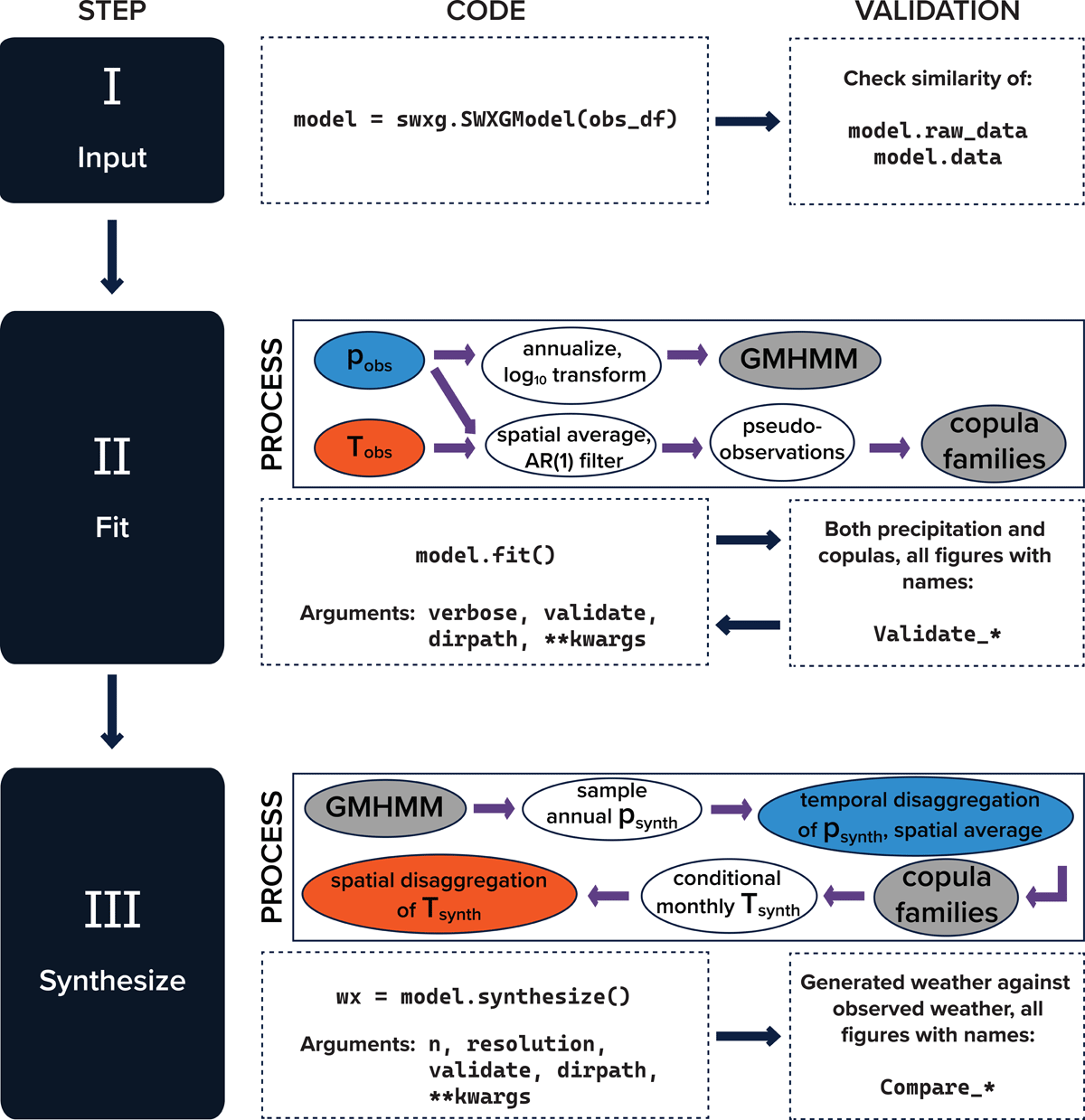
Figure 1
Generalized workflow—including the graphical and programmatic representation of critical methods, as well as arguments and validation checks—for the swxg library to move from input observations to generated weather. Workflow moves from left to right, top to bottom.
Figure 1 (I) represents the input step, in which the set of user-input observations is reworked into a data structure that the fitting models can accept. In order to do this, the input dataset (called obs_df in the CODE component of Figure 1 (I)) is expected to be in a pandas dataframe [45] with four columns:
SITE: The one or more locations in the region of interest for which there is hydroclimatic observations. Must have type str.
DATETIME: The temporal information about when each observation was collected. Must have type datetime64[ns].
PRECIP: The precipitation data. Must have type float in units of [m].
TEMP: The temperature data. Must have type float in units of [°C].
When attempting to input a dataframe into SWXGModel(), the class instantiation automatically checks that the input and each of its columns are of the right type, and will throw an AssertionError detailing the correct input if one of those types is incorrect. To better facilitate this, all arguments to all methods and functions that the user has access to have type hints included. After the correct format has been input, the SWXGModel() class formats the data by separating the DATETIME column into two or three columns depending on the temporal resolution of the input dataframe: YEAR, MONTH, and possibly DAY. This temporal resolution is recorded as an attribute of the model and can therefore take the values monthly or daily. While data at a subdaily resolution are accepted as input, as of this writing, generating at a subdaily resolution is not supported. After formatting, it is then recommended that the user guarantee that the original input dataframe obs_df matches the SWXGModel.raw_data attribute. Further, the user should also confirm that the temporal information has been successfully separated by comparing the number of rows in the SWXGModel.raw_data attribute with the number of rows in the SWXGModel.data attribute.
Figure 1 (II) represents the fitting step, in which the statistical models best representing both precipitation and the relationship between precipitation and temperature are applied. A graphical representation of this fitting procedure can be found in its corresponding Process section. Several required and keyword arguments may be passed to this method, with the most important of these being:
verbose: A flag for printing the precipitation and copula fit statistics to the screen so that they are not abstracted away, and the user must acknowledge how well the fit performed. This is enabled by default.
validate: A flag for creating all of the validation figures related to the fitting process. This is enabled by default. Figures validating the fit of a particular variable may be left on or turned off using the validation_figures keyword argument to better target analysis. All of the fit validation figures have a naming convention starting with Validate.
Users do not need to access any other method to perform the fit, and only need to give the fitting method the appropriate required and keywords arguments for their use case. Note that the fitting step is an iterative process, and users are recommended to refine the fit using keyword arguments.
The fit for precipitation is first calculated by aggregating the daily or monthly values to the annual resolution and applying a log10-transformation to the annual data. This has previously been found to be an appropriate model for streamflow [15, 17, 46, 47], and there is a strong dependency of streamflow on precipitation [48]. Then, a Gaussian mixture hidden Markov model (GMHMM), supplied by hmmlearn [49], is used to fit the transformed data and determine the appropriate number of (hidden) states, covariance and transition matrices, and statistical annual means and variances for precipitation, thus accounting for precipitation’s historical spatial correlations. The best-fitting number of states and best-fitting GMHMM model are determined by a comparison of log-likelihood, Akaike Information Criterion (AIC), and Bayesian Information Criterion (BIC) [50]. The default behavior is to use the BIC, but users have control over the best-fitting number of states. More information on how users can select their own number of states can be found in the Quality Control section.
The fit for the relationship between precipitation and temperature through copulas follows the approach outlined in [51]. The first step is spatially averaging precipitation and temperature across all of the sites to reduce the number of copulas to fit and therefore the overall model complexity. Next, an AR(1) filter [52] is applied to both the precipitation and temperature data to remove any autocorrelations that exist in the precipitation and temperature data. These AR(1) coefficients are then stored for later use. The residuals of this filter are then confirmed as stationary over the observation period using the augmented Dickey–Fuller [53] and Kwiatkowski–Phillips–Schmidt–Shin [54] tests. The residuals also confirm the dependence structure between precipitation and temperature using K-plots [55], which plot the expectation of the residuals’ order statistics under the null hypothesis of independence against the ordered empirical copula values. The K-plots in turn inform the appropriate copula family. The filtered monthly precipitation and temperature residuals are then converted to pseudo-observations (i.e., quantiles) through their empirical cumulative distribution functions (CDFs) and three possible families of copulas—Frank and Gaussian families to capture potential positive and negative relationships, and the independence family to capture potentially no relationship—are fit to each month. Additional families are being considered, but as of this writing have not yet been implemented; see the Discussion and Limitations section for more. The best-fitting copulas per month are determined by comparing the AIC and bootstrapped versions of the Cramér–von Mises criterion [56] and Kolmogorov–Smirnov test metrics [57, 58]; smaller values for each of these metrics represent better fitness of the copula family. The default behavior of swxg for each month is to choose the best-fitting family as the one that corresponds to two or more of the smallest metrics, and if there is no outright majority among the families, then the AIC alone is used. Users ultimately have the choice of default behavior or explicitly picking a copula family in the fitting method options. More information on this can be found in the Quality Control section.
Figure 1 (III) represents the generation step, in which the previously calculated and validated fits are used to produce novel time series of precipitation and temperature. A graphical representation of this generation procedure can be found in its corresponding Process section. Several required and keyword arguments may be passed to this method, with the most important of these being:
n: The number of years of weather data to generate. The default number of years to generate is the same as the input dataframe.
resolution: The temporal resolution of the generated weather. The default behavior is to have the same resolution as the input dataset; however, coarser resolutions are always possible (e.g., an input dataset of daily data can be used to generate monthly data). This is not true for finer resolutions, and if attempted, the method will return data at the input resolution.
validate: A flag for creating all of the validation figures related to the generation process. By default, this is enabled. All of the generation validation figures have a naming convention starting with Compare.
Users do not need to access any other method to perform the generation, and only need to give the generation method the appropriate arguments and keywords arguments for their use case.
swxg handles synthetically generating precipitation and temperature while maintaining historical spatial and temporal correlations by disaggregating the synthetic annual precipitation generated by the multivariate normal distribution. This is done by applying the method of fragments to a randomly selected historical year from the k-nearest neighbors, as done in prior studies [59, 60, 17]. This process yields a semiparametric generation of monthly precipitation, with the generation of annual precipitation being done parametrically and its disaggregation from annual to monthly precipitation being done non-parametrically. To conditionally generate monthly temperature from monthly precipitation, the monthly precipitation is spatially averaged across sites and filtered through the corresponding month’s stored AR(1) model to create synthetic precipitation residuals. These residuals are then transformed to pseudo-observations through the historical empirical CDF and input to that month’s copula. Temperature pseudo-observations (quantiles) are then conditionally sampled from the joint marginal probability at that value of the precipitation pseudo-observation. Finally, the temperature pseudo-observation is transformed back to a temperature residual using the inverse CDF of the spatially averaged temperature values, and then transformed to an actual temperature value using the inverse of its stored AR(1) fit. Collectively, this process results in a semiparametric, stochastically generated hydroclimate from a set of regional observations at the monthly resolution. If daily resolutions are desired, the same process as above is performed, with an additional step of using the selected k-nearest neighbor month and year to shift the daily observations (aggregated to the monthly resolution) to their synthetically generated monthly value. These daily observations are rescaled to their corresponding synthetically generated monthly value through a simple scaling factor determined by the ratio of the synthetically generated monthly value to the nearest-neighbor selected observed monthly value.
Quality Control
swxg has been successfully tested on Linux Ubuntu, macOS Sequoia 15, and Windows 11 with Python versions 3.10 and higher. It is also compatible within a Google Colab environment. Before using swxg for one’s unique case, users are advised to review the API in the accompanying documentation and follow a tutorial using the provided examples. There are two example datasets included in the library—accessible through the import paths swxg.test_wx.monthly and swxg.test_wx.daily. The daily dataset is demonstrated here, as the monthly dataset is presented and analyzed in [61]; the procedure for daily and monthly datasets is identical. The tutorial mirrors the procedure for an actual use-case and serves as a template for how to read in observations, how to interpret the goodness of fit for precipitation and temperature, how to refine the fitting, how to synthetically generate data from those fits, and how to confirm that the generated dataset and observed dataset are statistically indistinguishable. Note that not all figures produced by this library when validating the fits and the generated weather have been included in this paper. Further, while unnecessary for the test datasets, it is important to pretreat the input precipitation and temperature values before the initial fitting (e.g., fill in missing data). Help with data pretreatment is also available in the documentation.
The weather generation model can be instantiated and fit following the CODE components in Figure 1 (I) and (II):
model = swxg.SWXGModel(swxg.test_wx.daily)
model.fit()
Figure 2 shows a sample from the daily dataset, both as the raw input model.raw_data (a) and the formatted input model.data (b). It spans from 1 January 1968 to 12 October 2025 for two climate stations X and Y, and the one-to-one correspondence for row indices means that the instantiation of the model with the daily dataset was successful.
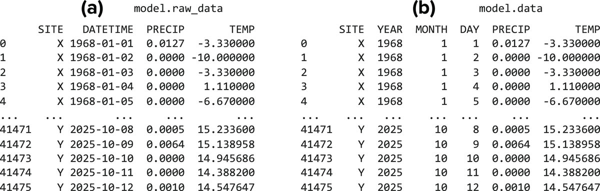
Figure 2
The daily dataset both as (a) raw input and (b) formatted input, where years, months, and days have been separated into their own columns.
Next, model.fit() produces the output seen in Figure 3. The topmost area of Figure 3 indicates whether or not a GMHMM fit has been found for the precipitation data using the corresponding number of states. In order to do this, a positive definite covariance matrix needs to exist. The comparison of the best-fitting number of states will include only the GMHMMs for which a positive definite covariance is found, even if more states were tried. The precipitation fit area in Figure 3 identifies what that best-fitting number of states was, the corresponding means and standard deviations of the discovered state(s) with their bootstrapped goodness of fit p-values using Anderson–Darling (AD), Cramér–von Mises (CvM), and Kolmogorov–Smirnov (KS) statistics [62], and the accompanying transition probability matrix for moving between states. The two rows of panels in Figure 4 show the fit scoring for each GMHMM model for each number of states and the normality of the log10-transformed annual precipitation data, respectively. Figure 4(a) plots the log-likelihood (yellow), AIC (blue), and BIC (green) vs. the number of states. Each of these metrics should be considered when validating the number of states; however, each metric is calculated differently and therefore evaluates the number of states differently. The log-likelihood metric is a good indicator of fitness for models with the same number of parameters, but it is often not a good metric for ranking models if they have varying numbers of parameters, as the value will monotonically increase with parameter number [63, 49]. It is included here to show that, indeed, more parameters do increase its value; if they did not, there would be a problem in the fitting. The AIC and BIC both penalize adding more parameters; however, they do so differently with the AIC penalizing per additional parameter (leading to possible overfitting) and the BIC penalizing per additional parameter and observation used in the fit (leading to possible underfitting) [64, 65]. Smaller values for both the AIC and BIC indicate better fitness. To be conservative in its fit assessment, swxg uses the BIC metric as the default choice to choose a best-fitting number of states, which in this case is a single-state GMHMM. Note that a single-state GMHMM reduces to a multivariate normal distribution. Data points closer to the red 45° line indicate data closer to theoretical normality, which is largely true for all data in Figure 4(b) and (c). The precipitation fits have now been validated, and users can include the precipitation-fitting keyword argument:
model.fit(kwargs={"gmhmm_states": 1})
to lock in the number of GMHMM states. If the user believes that the AIC was a better choice, they would replace the line above with:
model.fit(kwargs={"gmhmm_states": 3})
and then check the rest of the precipitation validation figures to confirm it. Note, if multiple states are chosen to be the best fitting, one Q-Q plot per state would be produced, with the observations per panel corresponding to each state. With three chosen states, there would be three Q-Q plot panels for site X and three for site Y, with each using the mean and variance of that state for the theoretical quantiles.
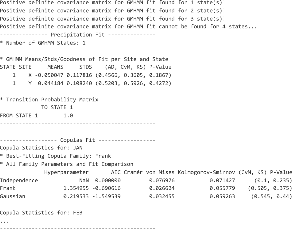
Figure 3
Initial fit statistics of daily data. No keyword arguments refining the fit have been used. Copula statistics for February through December have been truncated for this figure but will appear when run. Note that p-Value columns are bootstrapped and therefore may vary slightly between executions.
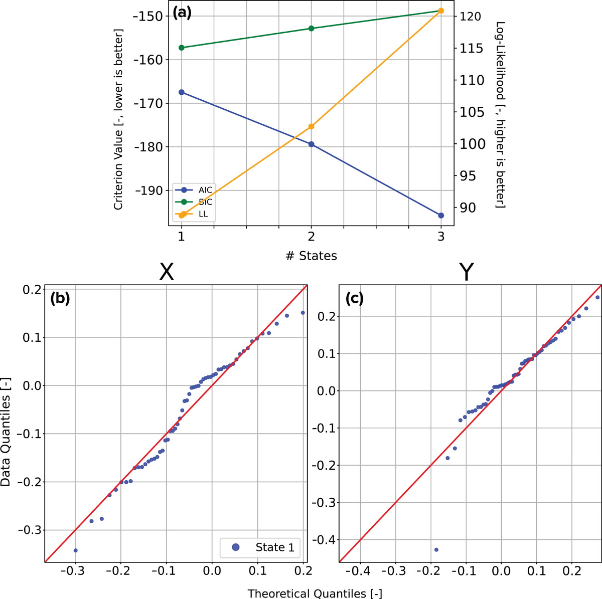
Figure 4
Validation of (a) the number of GMHMM states and (b–c) the normality of the log10-transformed annual precipitation data for both stations via Q-Q plots, using the best-fitting number of states based on BIC.
The Copulas Fit area identifies the scoring for each copula family—Independence, Frank, and Gaussian—applied to the spatially averaged observed precipitation and temperature data. These three families are considered because they each can represent positive, neutral, or negative relationships between marginal variables [51]. Figure 5 displays the AIC and bootstrapped versions of the Cramér–von Mises criterion and Kolmogorov–Smirnov test using the fits of each copula family for each month. Test metrics and their corresponding p-values are calculated following the procedures in [66]. Again, smaller values represent better fitness, and p-values are bootstrapped. Given that the independence copula takes no parameters, its AIC value is always exactly zero and represents a null hypothesis that precipitation and temperature are not correlated. Note that AIC values for all families within approximately two of each other are competitive interpretations [67]. To reduce model complexity, it is preferable to use a single copula family across all months, and because on average with this data, the Frank copula performs as good or better than the other families, the Frank copula is chosen as the best fit. If the fitness is markedly different by family, multiple families should be chosen. Figure 6 complements the quantitative assessment of best fit in Figure 5 with a visual assessment of each theoretical copula’s CDF (in two dimensions, shown in gray, blue, and red), compared to that of the empirical copula for the same monthly set of pseudo-observations in black. The lines themselves are the isolines of the CDF, and so the colored isolines that most closely follow the black isolines across each month represent the theoretical copula family that most closely matches the empirical copula. The Frank copula can also be seen across months in Figure 6 as being the closest fitting to the ‘true’ empirical copula. A best-fitting copula has now been identified, and users can include the copula-fitting keyword argument:
model.fit(kwargs={"gmhmm_states": 1,
“copula_families”: [“Frank”]})
to lock in the singular copula family. Critically, the user should now rerun model.fit() again using these arguments.
The re-fit model can generate precipitation and temperature following the CODE component in Figure 1 (III):
wx = model.synthesize()
Without any arguments, a dataset of synthetic weather will be produced of the same temporal resolution (in this example case, daily) with the same number of years as the original observation dataset (in this example case, 57). Figure 7 shows the possible realization of generated weather wx. Aside from different values in the precipitation and temperature columns relative to the input daily dataset, note two additional changes. The first is that the number of rows in the dataframe changed. This is because the generator produces a number of years equal to the difference between the first full year and the last full year, even if there is a partial or missing year between them. The second is that the values for each year changed. This is because the fits that each entry is generated from could apply to any year in any order, and so the first year in the generated set does not have a one-to-one correspondence with the first year in the observed set, and so forth.
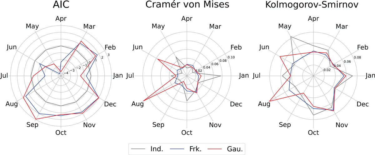
Figure 5
AICs (left), Cramér–von Mises criteria (middle), and Kolmogorov–Smirnov tests (right) for each copula family for each month. Families included are Independence (gray), Frank (blue), and Gaussian (red). Radially outward represents worse fitness.
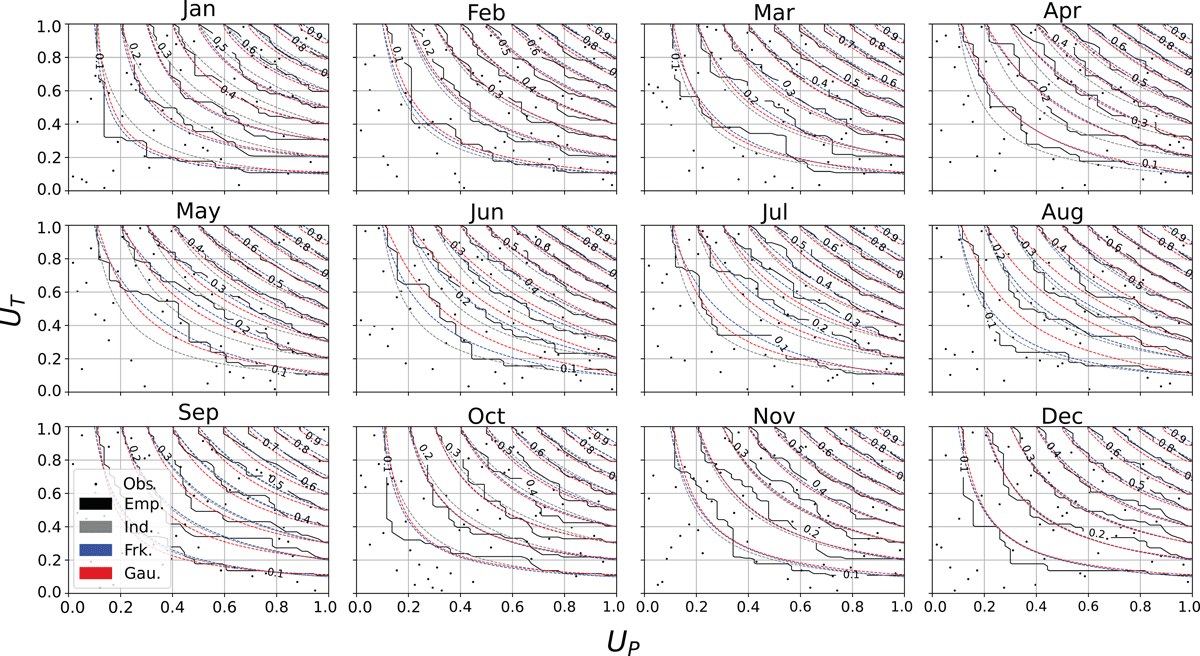
Figure 6
Theoretical copula families compared to the empirical copula (black lines) created from pseudo-observations of spatially averaged precipitation and temperature (black dots) for each month. Families included are Independence (gray), Frank (blue), and Gaussian (red).
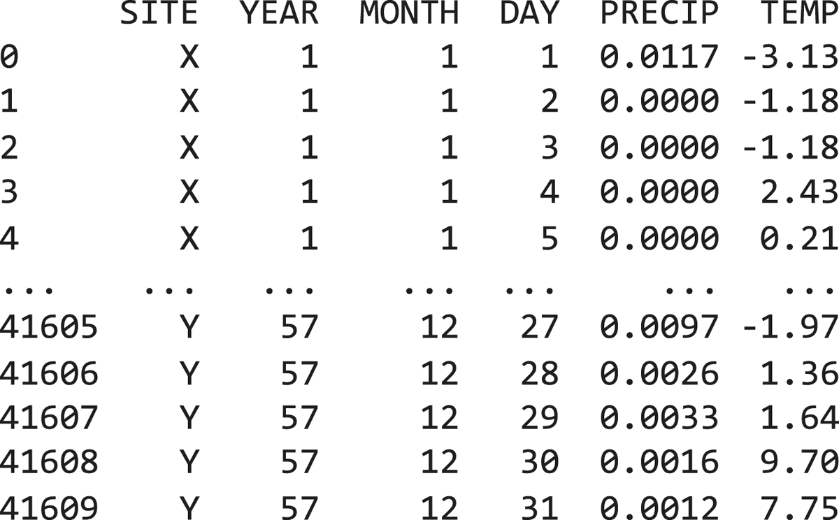
Figure 7
The generated dataset at the daily resolution. Values for precipitation and temperature are unique to this instance, but can be fixed by setting a local random seed.
A comparison of the generated and observed precipitation and temperature values for site X can be found in Figure 8. Exploring the internal variability of the daily dataset through its statistics shows that samples of the generated dataset (gray) both expand (scatterplot) in all dimensions around the historical observations (black) while maintaining the same underlying statistics (marginal histograms). The generator replicates these features across all months (and additional sites, which are not included for the sake of brevity). Figure 9 displays the spatial correlations between observed and generated precipitation and temperature for the month of January, while Figure 10 displays the fitness metrics for each month for site X corresponding to the observed and generated distributions in Figure 8. In Figure 9, the Pearson correlation coefficient is nearly the same for both observed and generated precipitation and temperature, indicating that the observed spatial correlations are reproduced in the generated set. In Figure 10, three two-sample tests are performed to assess different moments of the distribution: the Mann–Whitney U test [68], which tests for changes in the median; Levene’s test, which tests for changes in the variance [69]; and the Kolmogorov–Smirnov test, which tests for changes in the cumulative distribution [57, 58]. Accordingly, each bar represents whether or not the null hypothesis—that the observed and generated samples of precipitation and temperature come from the same distribution—can be rejected (below the dashed line) or cannot be rejected (above the dashed line). As all bars for both precipitation and temperature are above the dashed line, the null hypothesis cannot be rejected for any month at site X. Since there is no statistical difference between the generated and observed distributions of both precipitation and temperature, the generated weather represents a plausible sample of the system’s internal variability. Fits will be produced at the resolution supplied by the eponymous argument. At this point, with the generator fit, any new call to the synthesize() method will create a novel sample. The size of this sample can be controlled using the n argument, and the resolution of that sample can be controlled using the resolution argument. Help with saving and loading either the generated sequences or the generator itself is available in the associated documentation.
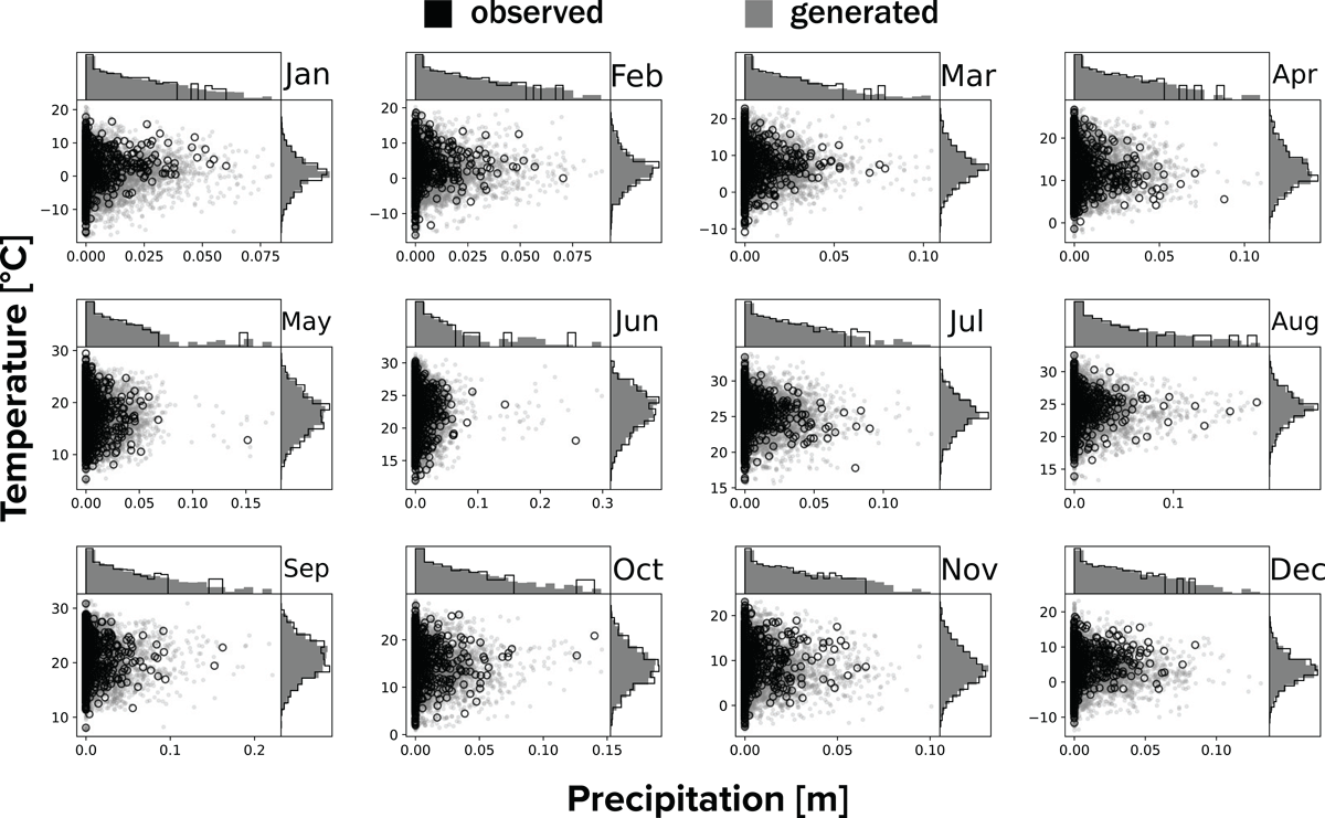
Figure 8
Statistical validation of synthetically generated precipitation and temperature across months for site X. Black symbols—open circles in the scatterplot and lines in the histogram—represent the swxg.test_wx.daily dataset from the years 1968–2025. Gray symbols—points in the scatterplot and bars in the histogram—represent the synthetic values sampled by the SWG.
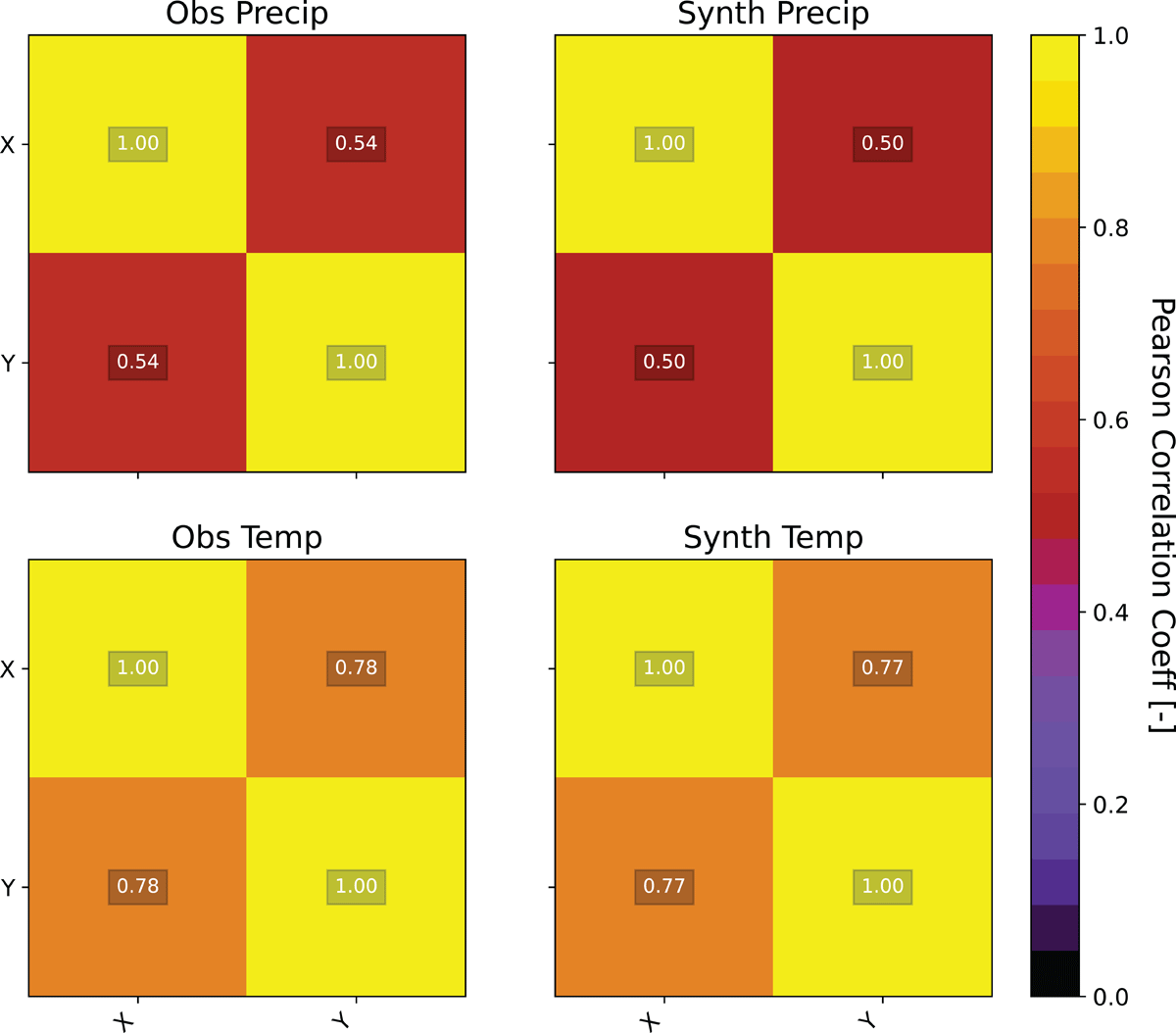
Figure 9
The preserved spatial correlations in the month of January between both observed and generated precipitation and temperature. Values centered in each box correspond to the color and value of the Pearson correlation coefficient. Note that the correlation across all months is symmetric, and the number of cells increases with the number of sites squared.
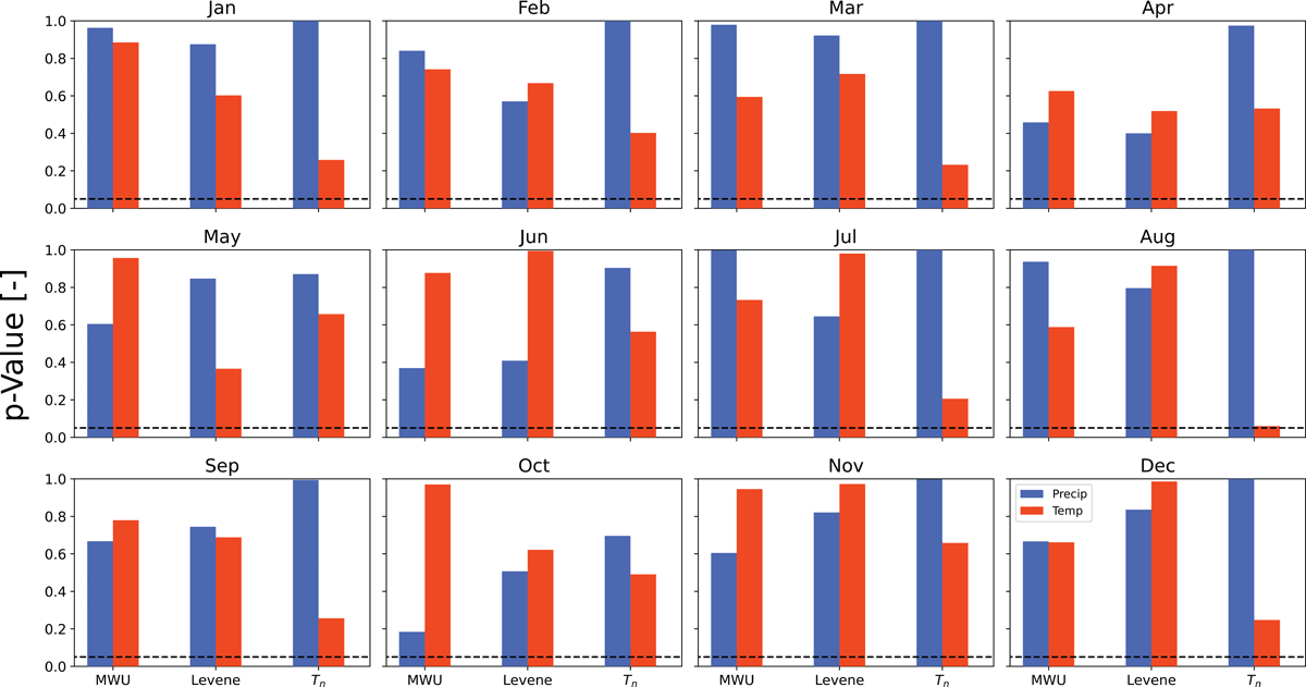
Figure 10
The complementary numerical fitness metrics plot to Figure 8. Each panel corresponds to a month at site X, and each color corresponds to either precipitation (blue) or temperature (red). Each test is listed on the x-axis, which are the Mann–Whitney U test (MWU), Levene’s test (Levene), and Kolmogorov–Smirnov test (Tn), and that test’s corresponding p-value is shown on the y-axis. Bars below the dashed black line represent those distributions for which the null hypothesis can be rejected.
Note that not all of the figures produced by swxg have been included in this manuscript (e.g., validation of spatial correlations between observed and generated data) as the number of figures scales with the number of sites; even with just two example sites, the total number of figures produced exceeds 35. A description of all figures produced by both fit() and synthesize() methods generally can be found in the accompanying documentation under the ‘How to Interpret Validation Figures’ page, while the figures produced specifically by the procedure outlined above can be found in the accompanying repository directory example_figures/.
(2) Availability
Operating System
Linux Ubuntu, MacOS Sequioa 15, and Windows 11 with Python versions 3.10 and higher. Additionally, Google Colab.
Programming Language
Python 3.10+, tested on Python 3.11
Additional System Requirements
N/A
Dependencies
The following dependencies are handled automatically during installation:
copulae >= 0.8
copulas >= 0.10, < 0.12
hmmlearn >= 0.3
matplotlib >= 3.8
numpy == 2.0
pandas >= 2.1
scikit-learn >= 1.4
scipy >= 1.15
statsmodels >= 0.14, < 0.15
These version numbers are such that the library behavior is consistent across testing environments, including Google Colab. As these internal dependencies are updated, these versions may be subject to change.
List of Contributors
All authors contributed to the software. Additional contributors are:
Ethan Heidtman: Testing alternate observations; Department of Geosciences, The Pennsylvania State University, University Park, PA 16802, USA.
Ava Spangler: Testing alternate observations; Department of Geosciences, The Pennsylvania State University, University Park, PA 16802, USA.
Software location
Archive
Name: Zenodo
Persistent identifier: https://doi.org/10.5281/zenodo.19320179
License: MIT
Publisher: Alexander B. Thames
Version published: 0.4.1
Date published: 12/11/25
Code repository
Name: GitHub
Persistent identifier: https://github.com/xthames/swxg/
License: MIT
Date published: 22/08/25
Language
English
(3) Reuse Potential
swxg is a flexible library that can be applied to any hydroclimatic or hydrological application where traces of the internal variability of precipitation and temperature across one or more sites are important outcomes to investigate. Further, the library can be used to validate the spatial and temporal correlations of observed and generated precipitation and temperature individually as well as jointly. Users interested in applying their own data to the generator should follow the procedures outlined herein and in the accompanying documentation. Users interested only in familiarizing themselves with weather generation techniques can simply import the library and use the included monthly- or daily-resolution datasets to learn through practice. A full description of the daily dataset has been provided in the Quality Control section, and this dataset represents observations collected near the mouth of the Susquehanna River at the Chesapeake Bay, USA. The monthly dataset, originally used in [61], represents observations collected west of the continental divide in Colorado, USA. Aside from the coarser resolution of the monthly data and the larger number of sites, there are no appreciable differences between the two datasets.
Discussion and Limitations
This paper has largely described how swxg—and by extension SWGs more broadly—can be used to synthetically generate samples of a system’s internal variability. However, in bottom-up impact and vulnerability assessments, addressing multiple states of the world (i.e., different underlying system statistics for precipitation and temperature) is just as critical as the realizations of the internal variability themselves. swxg is designed with this exploratory modeling [11, 12] extension in mind. Downscaled projections of future climatic conditions from repositories like [70] and [71] may also be used as inputs. To use these, the modeled historical climate accompanying the set of downscaled projections should be bias-corrected to match the historical observations of climate, after which the downscaled climate projections should be bias-corrected using these identified transformations [72]. The fits from these datasets can then be analyzed, and the ranges of model parameters of interest (e.g., precipitation mean/variance, copula hyperparameter, temperature mean/variance) can be extracted. A sampling scheme (e.g., orthogonal Latin hypercube [73, 74]) can then be applied to explore the parameter space, making sure to expand beyond the discovered ranges in order to capture both uncertainty and plausibility in the ranges as well as important interactions and mechanisms with consequential effects at and beyond the system’s initial boundaries [11, 15, 75]. The sampled, exploratory parameters can then be supplanted as the statistical fits to be used in this generator. This exploratory functionality thereby supports sensitivity analysis methods [76, 77, 78] as well.
At present, only Independence, Frank, and Gaussian copula families have been implemented in swxg. The Frank and Gaussian families allow for negative correlation structures, as is common between precipitation and temperature (55), and the Independence family reflects the null hypothesis that precipitation and temperature may be uncorrelated. Additional Archimedean copula families with asymmetric tails (e.g., Clayton, Gumbel) are not included in the release version of swxg as they can only support positive correlation structures between variables. However, the initial precipitation or temperature data could be negated to make negative correlations positive for copula fitting, which could be reversed again during synthetic generation. While this level of complexity is not yet included in swxg, upcoming versions are being developed to include these copula families with asymmetric tails.
Because swxg is at its core a statistical model, the quality of the input weather dataset will be reflected in (1) the confidence of the fits for precipitation and the copulas and (2) the resolution of the generated weather. For the former, to fit precipitation and the copulas, swxg aggregates precipitation and temperature at both annually and monthly scales, meaning that more complete years of input data will produce better fitting [79, 80]. A UserWarning will appear if you use fewer than 30 years of input data, which is our conservative lower bound on a sufficient sample size. A similar UserWarning will appear if more than 20 sites are used. While the fitting algorithm supplied by hmmlearn does not list any known computational or statistical issues for an arbitrarily large number of sites, the time for the algorithm to converge on a positive definite covariance matrix may exceed its default walltime. Accordingly, users have control over this walltime using the max_convergence_attempts keyword argument in fit(). In both cases, fitting will proceed regardless, but it is strongly recommended to validate the precipitation and copula fitness through additional metrics if either condition is met. For the latter, when generating weather swxg gives the option to determine its output resolution, either at the monthly or daily scale. How resolved the generated weather can be is determined by the input dataset: monthly inputs can be resolved to monthly outputs; daily inputs can be resolved to both daily and monthly outputs. A UserWarning will appear when trying to resolve daily outputs from monthly inputs. If attempted, the monthly resolution will output instead. Subdaily inputs are accepted but as of this writing generating at the subdaily scale is not yet implemented, and so subdaily data are aggregated to daily.
Acknowledgements
The authors acknowledge the Penn State Institute for Computational and Data Sciences for computational resources.