
(1) Overview
Introduction
The scientific-computing community uses numerical solvers implemented in different programming languages, such as C, C++, Julia, Python, or R. In addition to that, each solver has its own programming interface in terms of function names, order of arguments, and the order of function invocation. Due to these two factors, interoperability is inhibited, as switching from, say, a solver for initial-value problems for ordinary differential equations from the SciPy package [27] to another solver implemented in C, such as the SUNDIALS suite [1014], requires significant effort from computational scientists. First, bindings between two languages must be written for a particular numerical library, which is a nontrivial task, even when software packages such as Cython [25] or pybind11 [29] can decrease the required workload by partially automating the procedure. However, the second factor—different programming interfaces in different implementations—must also be addressed, which requires writing additional code and testing. Moreover, usually such efforts remain coupled to the actual project, without considering open-sourcing it, so that multiple computational scientists must redo the same work.
To alleviate these difficulties, we work on software Open Interfaces with two layers. First, we develop a set of generic interfaces for typical scientific-computing tasks (such as integration of ordinary differential equations), which are used to abstract out discrepancies between different implementations of these algorithms. These interfaces are written in a uniform manner across supported programming languages from a single specification (currently manually with planned automatic generation in the future). Second, we develop a mediator library that automates passing data between different languages so that writing explicit bindings is not required. Therefore, computational scientists could switch more easily from one implementation to another, while working through the same programming interface, which leads to faster time-to-solution and eases the usage of these implementations for less programming-inclined scientists as fewer code modifications would be required.
The ideas behind the Open Interfaces are the idea of programming against an interface and the idea of unifying different numerical solvers under a single interface using the Adapter pattern of object-oriented programming [8] and drive the software design of multiple numerical packages. Although the ideas themselves are not new—an early and perhaps the most prominent example in numerics is Basic Linear Algebra Subroutines (BLAS) [19] published in 1979— they have gained significant popularity in scientific computing in recent years [5] and drive software design of multiple modern numerical packages. Some further examples are the pyMOR package by Milk et. al. [22] for model-order reduction with the Python programming language, with the algorithms interacting with full-order models in terms of abstract vector operations allowing the package users to write new models in other languages or reuse existing PDE solvers, e.g., DUNE [28], deal.II [1], NGSolve [9]. Chourdakis et al. [6] developed library preCICE written in C++ with bindings to other popular languages that allows users to couple a wide spectrum of finite-elements and finite-volume solvers, such as FEniCS [2], and OpenFOAM [34] for multiphysics simulations, providing facilities for communication, data mapping, and interpolation between the solvers. The Earth System Modeling Framework [13] provides unified interfaces to different components needed for geophysical and weather simulations. The software package UM-Bridge [2324] provides a general way of decoupling algorithms and models for Uncertainty Quantification problems via wrapping models in a container and accessing them only via HTTP protocol, enabling users of languages like C++, Python, R, and Julia to access models written in different languages.
The main distinction between the aforementioned projects and Open Interfaces is that we concentrate on common basic problems in Applied Mathematics in contrast to, e. g., preCICE that provides components in the domain of structural-mechanics and fluid-dynamics simulations. Another difference is that some of these projects focus on a subset of languages popular in Scientific Computing: for example, pyMOR’s target language is Python, while the Earth System Modeling Framework provides bindings only for Fortran and C. Open Interfaces, on the other hand, strive to treat all programming languages on the user’s side as equal, without forcing the users to use a particular one.
The software package in its current status defines an interface for solving initial-value problems for ordinary differential equations (time integration) and realizes this interface on the user side for the C and Python programming languages, with implementations from the SUNDIALS, SciPy, and OrdinaryDiffEq.jl packages. Already useful in this state, the package demonstrates what can be achieved in terms of crossing the language barrier and using different solvers for the same problem type via the interface for time integration.
For further development, we plan to define a formal interface specification language and auto-generate corresponding code (wrappers for users to invoke implementations, abstract base classes, etc.) for all supported languages. We will increase the number of available interfaces and corresponding supported implementations with other common numerical tasks, such as optimization. Also, while we currently concentrate on in-process computations, where the data are passed from the user to an implementation as pointers, we also plan to extend the available transport methods to remote-procedure calls, similar to UM-Bridge, for problems, in which the overhead of copying data between processes is negligible.
Implementation and architecture
In this section we describe the Open Interfaces library, with the following principles guiding the software architecture.
The main organizational principle is decoupling of user’s code from a numerical implementation (which can be written in a different language). The second organizational principle in the architecture is the use of the C programming language [16] for intermediate representation of the data and core libraries that decouple interfaces from implementations. Last, the aim to preserve performance as much as possible. In the following subsections we expand on these principles in details.
Architecture, data flow, and realization details
As was stated before, we decouple users and implementations from each other. Precisely, we strive to avoid direct pairwise connections between programming languages on the user side and the implementation side by inserting a mediator library (which we refer to as liboif) which allows reduce the amount of work required by computational scientists with different preferred languages, such as C, Julia, or Python, to use numerical libraries, which can be also written in different programming languages.
Indeed, as Figure 1 shows schematically, with L languages and I implementations, one needs 𝒪(L×I) amount of work in case of pairwise connections, while only 𝒪(L+I) connections via the mediator library liboif.

Figure 1
Schematic comparison of two approaches to the problem of multiple languages/multiple implementations. A Standard pairwise bindings, B Bindings via Open Interfaces (OIF).
This library is actually a set of libraries that automate data marshalling (i. e., data passing) between different languages and dispatch function calls from the user to the user-requested implementation. Figure 2 shows the architecture of the library with the data flow from left to right from the user to a numerical solver. The vertical lines denote the boundaries between distinct components of the software organization.
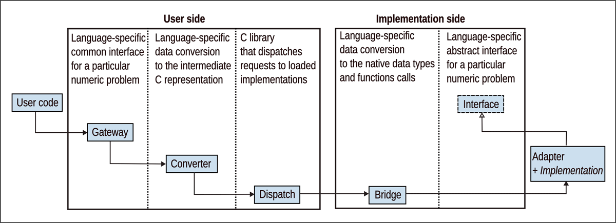
Figure 2
Data flow from user to implementation in MaRDI Open Interfaces.
The components on the “User side” are the components that users interact with directly such as an interface for a given numerical problem, or the components that are stable in a sense that they are belonging to the library itself and realize operations such as data conversion and loading implementations.
Components on the “Implementation side” are the components that call implementation methods via provided interfaces. Particularly, this means that for existing implementations, an adapter must be written that translates the calls from Open Interfaces to the calls that the implementations understand. Formally, such adapters and implementations themselves are not components of the library.
The responsibilities of each component of the system are the following:
Gateway provides an interface for a particular numerical problem, through which users can interact with multiple implementations. In OOP languages, it also automatically loads/unloads implementations in constructor/destructor, while in non-OOP languages it is the responsibility of the user.
Converter converts native data types to intermediate C representation and passes these data further to the Dispatch component.
Dispatch finds the requested implementation on disk, reads implementation details, such as the language, instantiates the Bridge component for this language (if not already instantiated), passes implementation details to it, such as module names in Python or shared library name in C, and saves the loaded implementation in the table.
Bridge loads an Adapter (along with the implementation) from the implementation details, calls implementation methods converting data from intermediate C representations to the native data types for the implementation language, and finally unloads it (when requested by the user).
Interface provides an interface that implementation adapters must implement. This component is an abstract interface defining the functions signatures, that is, it does not have any functionality itself.
Adapter does not belong to the library but only implements the interface described by an Interface component. It translates method calls from Open Interfaces to the implementation.
Note that the number of the Gateway and Interface components is equal to the number of the provided interfaces for numerical problems multiplied by the number of supported languages: they must be predefined for each problem type and match each other (at the present time we write them by hand with a plan to use automatic generation in the future); the number of the Converter and Bridge components is equal to the number of supported programming languages on user and implementation sides, respectively; the Dispatch component is a singleton that is oblivious of the languages it connects on both sides as well as the supported problem types.
To understand the workflow better, let’s consider three main phases of interaction between the user and Open Interfaces. In initialization phase, the user specifies what interface they want to use along with the string identifier for the needed implementation. In the calling phase, the user interacts with the implementation through the Gateway instance, which is a class in object-oriented languages like Python, or a set of functions in languages like C and Julia. When the user is finished using a particular implementation, this implementation is unloaded in the unloading phase.
Initialization phase. Figure 3 shows the UML sequence diagram of function calls that occur in the initialization phase. The user creates a Gateway component for a particular interface, passing a string identifier for the needed implementation of that interface. Gateway passes information about the interface and the implementation to the Converter, which converts this information to two C strings. These strings are passed to the Dispatch component, which first finds on disk the implementation details from the data pair “interface-implementation”. The details are language-specific, so that Dispatch itself only processes the first chunk of the details—the language—and loads a corresponding Bridge component (if it is not loaded before). The Bridge component processes the rest of implementation details (which are names of shared libraries in C, or Python modules, etc.) and loads the Adapter itself, which in turn loads the implementation.
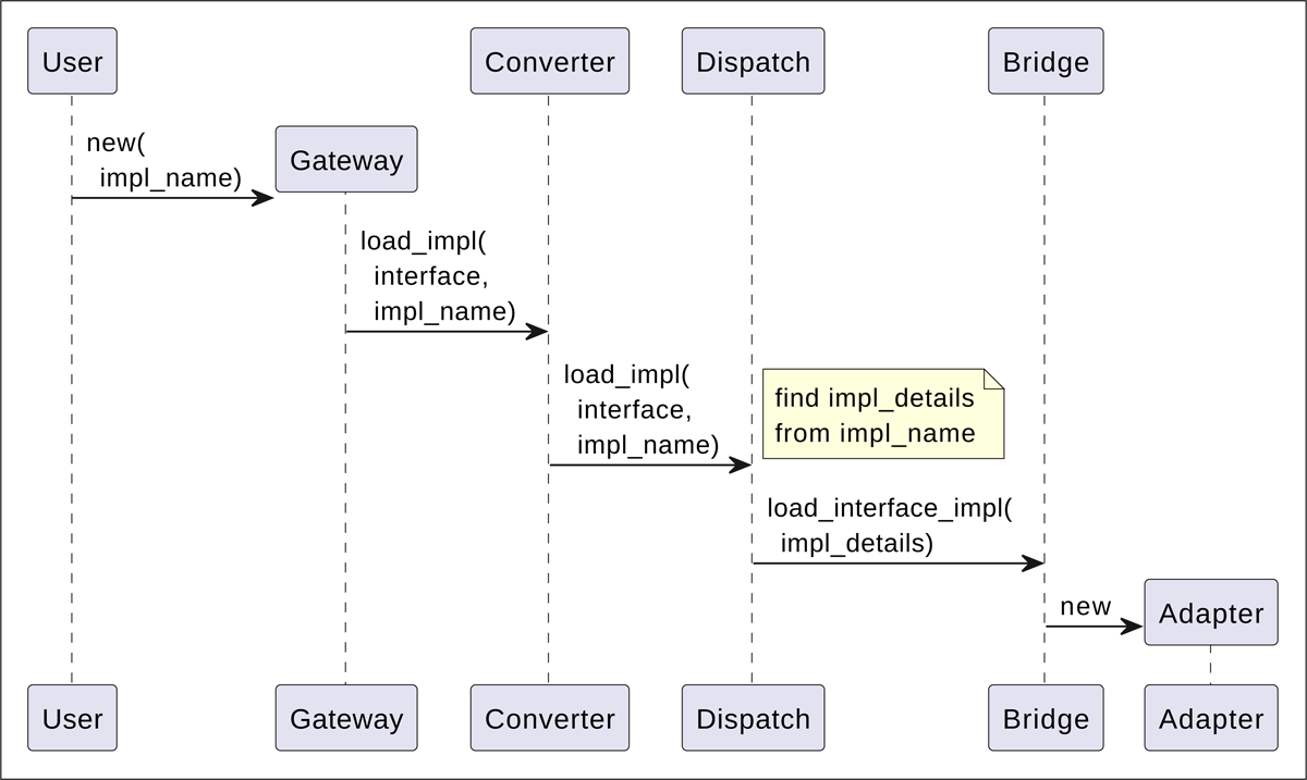
Figure 3
UML sequence diagram for the initialization phase, in which user requests an implementation for an interface of interest. The abbreviation “impl” stands for “implementation”.
At the end of the initialization phase, the user holds an implementation handle implh (implicitly in object-oriented languages such as Python or explicitly in languages such as C), which further acts as the identifier connecting all components together. Additionally, the Dispatch component saves the initialized implementation in the table of loaded implementations: the instantiated Bridge and the loaded implementation, which can contain multiple pieces of information, depending on the language, in which it is written. For example, it can be a loaded shared library in case of C or instantiated object in Python. Besides that, for non-OO languages, abstract state information can be also preserved in this table, which is determined by a particular implementation’s needs.
Calling phase. Figure 4 shows the generic sequence of function calls through the system when the user does the actual numerical computations. Each function call from the user to the Gateway is passed further to the Converter that packs different arguments into a list with each argument converted to its C representation and passes the implementation handle, the interface method name and the packed arguments to the Dispatch component. The Dispatch component does here only minimal work: it finds the record in the implementation table and passes the information further to the corresponding Bridge component. The Bridge component unpacks the arguments from the list and transforms them to the native data types of the language, and then invokes the requested method on the Adapter component. The Adapter component does the computations by using the implementation.
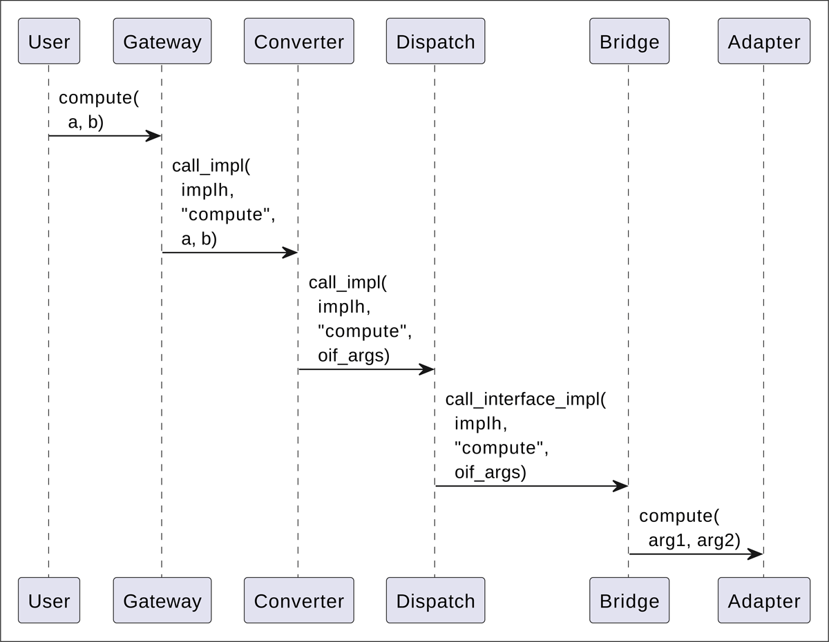
Figure 4
UML sequence diagram showing the function invocations when the user does the actual computations. The diagram shows invocation of a hypothetical method compute with two arguments that are converted to a list oif_args and then unpacked by the Bridge component to native data types of the implementation.
To simplify memory management, we strive to have all necessary memory allocations done on the user’s side, explicitly by the user or inside the Gateway component. However, in general this is not always possible, and in such cases the memory ownership must be explicitly pronounced in interface definitions, to diminish the possibility of memory leaks.
Unloading phase. When the user has finished using the implementation, it is unloaded from the memory as shown in the Figure 5. Precisely, when the user deletes the Gateway component (in an OO language like Python), the request to unload the implementation is executed automatically, while it must be executed explicitly by the user in languages like C. When the Dispatch component processes this request, it removes the implementation from its table and releases all memory related to the implementation.
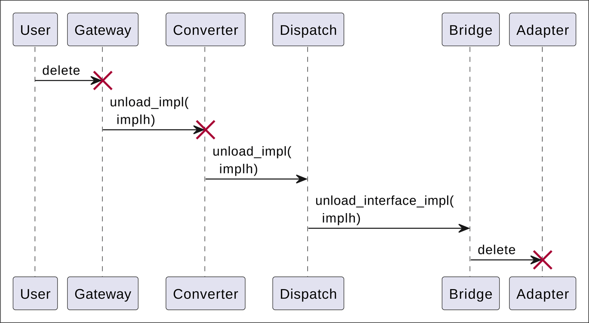
Figure 5
UML sequence diagram showing the function invocations for the unloading phase when the user has finished using the implementation.
Note that, as shown in the Figure 5, the Dispatch component is not deleted, as it still continues to keep the implementation table. The Bridge is not deleted either as, for example, the embedded Julia interpreter cannot be started again after finalization.
Data types
As stated before, we use C data types for intermediate representation, as popular languages used in scientific computing, such as Python and Julia, have facilities to communicate with C and making function calls to C, providing means of conversion of the data from the intermediate representation to the native data types of these languages.
Particularly, it is easy to convert Python and Julia integer data types to C int data type, provided that the integers are representable in 32 bits. Also, conversion of binary double-precision floating-point numbers is straightforward between C and other languages due to the widespread use of the IEEE 754 standard for floating-point arithmetic [15].
Data marshalling of arrays of double-precision floating-point numbers is made possible by using an auxiliary data structure OIFArrayF64 that, similarly to NumPy arrays [12] or Julia arrays, represents n-dimensional array for given n∈ℕ and packs data together with the number of dimensions n and the array shape, that is, the size of the array along each dimension. This data structure enables a uniform function signature among supported languages (currently C, Python, and Julia) as then the arrays are given as a single function argument in all these languages (in contrast with traditional use of C arrays, where data and dimensions are provided as separate arguments). Correspondingly, we use NumPy C API and Julia C API to convert to OIFArrayF64 and back when needed.
We also support read-only strings that can be used to pass information such as, e. g., a name of an integrator.
As it is common in scientific computing to pass callback functions to numerical solvers, Open Interfaces support passing functions between different languages. This is achieved in the following manner. Additional data structure OIFCallback is used that encodes information about the original language of the callback function, the function itself in this language, and the C-compatible version of this function. Consequently, on the language-specific dispatch level, if the user-facing and implementation languages are the same, the original callback function is used to avoid performance penalties, while the C-compatible callback is wrapped in the programming language of the implementation.
Additionally to the callback, passing a generic memory pointer is supported which is required, for example, to pass context to the callback functions. Although in languages like Python one can simply use closures to pass the context, in languages like C it is the only way to achieve this.
Finally, simple dictionaries of key-value pairs, where keys are strings, and values are either integer or floats, are supported to pass generic options that are implementation-specific.
For each supported data type, the data are passed between software components along with integer identifiers allowing to restore the type on the receiver end. We use the following symbolic constants further in the text to refer to the actual data types:
OIF_INT: 32-bit integers,
OIF_FLOAT64: 64-bit binary floating-point numbers,
OIF_ARRAY_F64: arrays of 64-bit binary floating-point numbers,
OIF_STR: strings with one-byte characters
OIF_CALLBACK: callback functions,
OIF_USER_DATA: user-data objects of volatile type,
OIF_CONFIG_DICT: dictionary of key-value options pairs.
It is assumed that each symbolic constant is replaced with the actual data type when used in a particular language: for example, OIF_ARRAY_F64 resolves to the provided data structure OIFArrayF64 in C and to NumPy arrays with dtype=numpy.float64 in Python.
Data passing and function calls
Copying data, especially, large arrays, impedes performance, as modern computer architectures are bounded by memory operations. Hence, in development of Open Interfaces, we avoid copying data and pass all data as pointers, which makes all conversion operations fast and cheap. Conversion of integer and floating-point numbers is cheap by itself, but even for arrays, it is a matter of creating a thin wrapper around an actual data pointer.
To invoke functions between different languages, the libffi1 library is used, either indirectly, e. g., using ctypes in Python, or explicitly for calling C functions dynamically.
Note that we use C convention of functions returning an integer to indicate an error. When the resultant integer is zero, the function invocation is successful, and not otherwise. For languages that support exceptions, an exception is raised on the user side, so that the user does not have to check every function call for errors.
Interface for initial-value problems for ODEs
One of the use cases already developed in this project is the open interface for solving initial-value problems (IVP) for ordinary differential equations (ODEs), namely, for problems of the form:
where , , y0 is the initial system state at time t0. We refer to this interface as IVP in the following text.
This interface, in a C-like pseudolanguage, consists of the following function invocations:
// Set an initial condition
OIF_INT set_initial_value(OIF_ARRAY_F64 y0, OIF_FLOAT64 t0);
// Set the right-hand side (RHS) callback function
OIF_INT set_rhs_fn(OIF_CALLBACK rhs_fn);
// (Optional) Set relative and absolute tolerances
OIF_INT set_tolerances(OIF_FLOAT64 reltol, OIF_FLOAT64 abstol);
// (Optional) Set user-defined data that are passed
// to the right-hand side function
OIF_INT set_user_data(OIF_USER_DATA user_data);
// (Optional) Set integrator and its parameters
OIF_INT set_integrator(OIF_STR integrator, OIF_CONFIG_DICT params);
// Integrate to new time and write the solution to vector y
OIF_INT integrate(OIF_FLOAT64 t, OIF_ARRAY_F64 y);
This interface assumes that the right-hand-side (RHS) function has the following signature: OIF_INT rhs_fn(OIF_FLOAT64 t, OIF_ARRAY_F64 y, OIF_ARRAY_F64 ydot, OIF_USER_DATA user_data), where ydot is the output variable to which the value of f(t,y) is written.
Quality control
MaRDI Open Interfaces uses testing and continuous integration for quality control. The test suite includes tests for all supported languages on the user’s side and assesses the behaviour of all included implementations against problems with known analytical solutions, with additional tests against edge cases such as wrong input. Further, unit tests for checking internal data structures and functions are also included. The test suite is based on standard tools for corresponding languages, such as Google Test2 for C and pytest [17] for Python.
Additionally, we use continuous integration service provided by GitHub that regularly runs the tests as well as static analyzers and style checkers, ensuring that the software’s results are reproducible and correct and that the code style remains consistent.
To help users learn the package, we provide documentation3 for the most recent release, with instructions on installation, how to check that the compiled package works as expected by running tests, and how to get started using the package with several examples. The full source of these examples is provided in subdirectory examples of the source code.
Examples
We explain shortly in this section a couple of examples of using the software along with the outputs.
Solve Burgers’ equation from C
The first example is solving in C inviscid Burgers’ equation:
after converting it to a system of ordinary differential equations:
where U(t) is a grid function discretized on a finite-volume grid of resolution N. To solve this system, we approximate fluxes at the finite-volume interfaces xi–1∕2, , using the global Lax–Friedrichs flux [20]. We integrate the system (2) to final time 10.
We use the C version of the IVP open interface for integrating in time, but for brevity omit checking error status codes here. First, we initialize a desired implementation (which is in the variable impl) of the IVP interface:
ImplHandle implh = oif_init_impl('ivp', impl, 1, 0);
and after the initialization, the user obtains an implementation handle implh that is used in all subsequent function calls. Note, that the third and the fourth arguments of the function oif_init_impl are for specifying the version of an implementation, however, right now this numbers are not used.
Now, we allocate a vector y for the solution of size N, set initial conditions (y0 at time t0), user-provided right-hand side callback rhs, and user data (context) that must be passed to the right-hand side callback (in this case, spatial step dx)—all this information is derived from Eq. (2):
OIFArrayF64 *y = oif_create_array_f64(1, (intptr_t[1]){N});
status = oif_ivp_set_initial_value(implh, y0, t0);
status = oif_ivp_set_rhs_fn(implh, rhs);
status = oif_ivp_set_user_data(implh, &dx);
Finally, we integrate the system for desired number of steps n_time_steps using uniform time step dt:
for (int i = 0; i < n_time_steps; ++i) {
    t = t0 + (i + 1) * dt;
    status = oif_ivp_integrate(implh, t, y);
}
Note that due to the lack of object-orientation in C, the user must keep the handle to implementation implh and pass it to every function of the IVP interface.
Figure 6A shows the solution of the problem (2) obtained using the dopri5 integrator (Dormand-Prince 5(4) method) from the scipy_ode implementation, which is an adapter to the SciPy package.
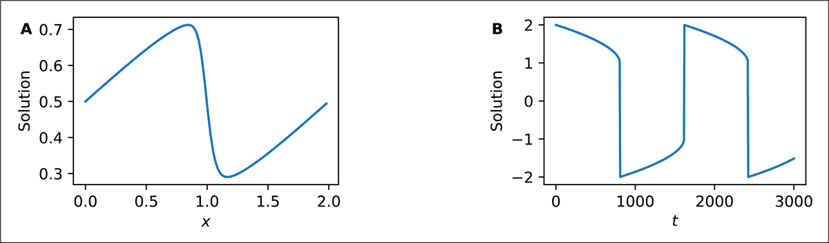
Figure 6
Example solutions obtained using MaRDI Open Interfaces: A Solution of the problem (2) using scipy_ode implementation with integrator dopri5 (Dormand–Prince 5(4) method). B Solution of the problem (3) using jl_diffeq implementation with integrator Rosenbrock23.
The full code of this example can be found in the repository at the path examples/call_ivp_from_c_burgers_eq.c.
Solve Van der Pol’s equation from Python
In the second example, we use Python and solve the Van der Pol’s oscillator equation:
with μ = 1000. The problem (3) can be converted to a system of first-order ODEs and solved again using the IVP open interface. However, due to the value of the parameter μ, the system is stiff and the system must be solved using implicit ODE solvers [20].
Indeed, if we try to solve the system using, for example, scipy_ode IVP implementation, which by default uses the Dormand–Prince algorithm [7]:
p = VdPEquationProblem(mu=1000, tfinal=3000) # User class
s = IVP('scipy_ode')
s.set_initial_value(p.y0, p.t0)
s.set_rhs_fn(p.compute_rhs)
then the computations fail due to stiffness:
UserWarning: dopri5: problem is probably stiff
Switching to the jl_diffeq implementation that adapts Julia’s OrdinaryDiffEq.jl package to the IVP interface of Open Interfaces, one can choose one of the implicit solvers that solve the problem (3) efficiently:
p = VdPEquationProblem(mu=1000, tfinal=3000) # User class
s = IVP('jl_diffeq')
s.set_initial_value(p.y0, p.t0)
s.set_rhs_fn(p.compute_rhs)
s.set_integrator('Rosenbrock23')
where Rosenbrock23 is a Julia’s implementation of the MATLAB’s ode23s integrator [26]. The integrator succeeds, with the solution shown in Figure 6B.
The full code of this example is available in the source code repository at the path examples/call_ivp_ from_python_vdp.py.
Performance analysis
To assess the performance loss that might be introduced by the core components of the Open Interfaces, namely, components that convert data and dispatch function calls, we conduct performance comparison using different combinations of user languages and implementations.
All run time results in this section are reported as 95% confidence intervals based on a sample of runtimes , n = 30, with sample mean
and the standard error of the mean
The performance study is based on time integration of Problem (2).
The runtime can be heavily affected by the performance of the used time integrator and the performance of the RHS evaluation, and we try to make sure that these two factors are of the same magnitude between different implementations.
For all implementations we use the Runge—Kutta 5(4) method of [7] with relative and absolute tolerances set to 10-6 and 10-12, respectively. The first implementation is in C and is translated from the original code from [11], and we refer to it in the further text as DOPRI5-C. The second implementation is in Julia, from the OrdinaryDiffEq.jl package, from which we use the integrator DP5. The third implementation is from Python’s SciPy package, from which we use the integrator DOPRI5 (which is actually written in Fortran [11]).
We also make sure that the RHS implementations have similar performance across all languages. To do that, we optimize by hand. Additionally, we compile the C RHS implementation as a shared library using the Clang compiler [21] and optimize the Python RHS version using Numba [18]. Thus, all versions of the RHS function are compiled to machine code via LLVM compiler infrastructure.4 Table 1 shows the run times, in seconds, of evaluating RHS implementations 10000 times for . As the data show, all RHS implementations have similar performance. These performance experiments were conducted using a workstation with an Intel Xeon E5-1630 v3 processor and 32 gigabytes of memory.
Table 1
Runtimes, in seconds, of evaluating RHS implementations for system (2) 10000 times at resolution .
| IMPLEMENTATION LANGUAGE | RUNTIME, SECONDS |
|---|---|
| C | 0.115 ± 0.008 |
| Julia | 0.122 ± 0.016 |
| Python (Numba) | 0.116 ± 0.001 |
Table 2 shows the results of the performance study. We run simulations for three different resolutions and compare different combinations of user languages and implementations. The table consists of three blocks corresponding to three comparisons.
Comparison 1. First we compare performance of time integration using the implementation DOPRI5-C invoking it via Open Interfaces and directly. As can be seen, performance penalty is small as for all used resolutions the run times do not differ for more than six percents.
Comparison 2. Here we compare run times of using the DP5 implementation from C via Open Interfaces against using the same DP5 implementation from Julia directly. In this comparison, the first two cases use the C RHS implementation, while in the third case the Julia RHS implementation. We can see that for N = 1600 there is a performance penalty of 20–50% because of invoking DP5 from C, that is, for this resolution, the overhead of Open Interfaces is non-negligible. However, already for moderate resolution N = 6400 the difference in runtime is not more than 5%, and for it is less than 2%. Between the first and the third cases in this comparison, the first case, with the C RHS via Open Interfaces, is slightly faster than the third case, with the Julia RHS and direct invocation of the DP5 solver, which is expected, as the C RHS is slightly faster itself than the Julia RHS (see Table 1).
Comparison 3. In this comparison we consider user code implemented in Python, with the RHS functions optimized via Numba, and run two implementations—DOPRI5 from SciPy and DP5 from OrdinaryDiffEq.jl—via Open Interfaces and directly. We can see that there is practically no runtime difference between using the DOPRI5 implementation from Python codes directly or via Open Interfaces. If the DOPRI5 implementation from SciPy is replaced with the integrator DP5 from the OrdinaryDiffEq.jl package, the runtime is 73% longer for , 6% shorter for and 9% shorter for , which suggests that OrdinaryDiffEq.jl solvers are more performant than SciPy solvers, although for smaller resolution there is clear overhead of using Open Interfaces. Longer runtimes for the Python code, relative to the C and Julia codes used in Comparisons 2 and 3, were influenced by the performance of the Python interpreter.
Overall, we can see from these three comparisons that the performance penalty of Open Interfaces is on average less than 5% for significant workloads.
Lack of a Gateway and Convert components in Julia at the current stage of the project has prohibited us from conducting a comparison for Julia user codes, however, we expect that the results of such a study would not change the results demonstrated in Table 2.
Table 2
Run times, in seconds, of time integration of system (2) using different user languages: C, Julia, or Python, with “Julia (C)” meaning that RHS implementation is in C), different ways of invoking implementations: via Open Interfaces (OIF) or directly (RAW), and three different implementations (DOPRI5-C—C translation of the original Fortran code [11], DP5 from Julia’s OrdinaryDiffEq.jl package, DOPRI5—Python wrapper over the original Fortran code [11] from SciPy).
| # | USER LANGUAGE | OIF/RAW | IMPLEMENTATION | N | ||
|---|---|---|---|---|---|---|
| 1600 | 6400 | 25 600 | ||||
| 1 | C | OIF | DOPRI5-C | 0.068 ± 0.001 | 1.011 ± 0.017 | 21.006 ± 0.100 |
| C | RAW | DOPRI5-C | 0.069 ± 0.001 | 0.951 ± 0.012 | 20.699 ± 0.121 | |
| 2 | C | OIF | DP5 | 0.082 ± 0.000 | 0.847 ± 0.003 | 20.700 ± 0.049 |
| Julia (C) | RAW | DP5 | 0.056 ± 0.002 | 0.820 ± 0.008 | 20.364 ± 0.073 | |
| Julia | RAW | DP5 | 0.067 ± 0.009 | 0.868 ± 0.004 | 21.058 ± 0.067 | |
| 3 | Python | RAW | DOPRI5 | 0.113 ± 0.000 | 1.573 ± 0.010 | 30.829 ± 0.121 |
| Python | OIF | DOPRI5 | 0.122 ± 0.009 | 1.575 ± 0.005 | 30.944 ± 0.122 | |
| Python | OIF | DP5 | 0.196 ± 0.003 | 1.466 ± 0.005 | 28.147 ± 0.040 | |
(2) Availability
This package does not impose any requirements on an operating system but requires a Unix-like environment.
Programming language
Package building requires a C17+ compiler. During runtime, Python 3.11–3.13 and Julia 1.11+ are needed for corresponding implementations.
Additional system requirements
None
Dependencies
All mandatory dependencies include a C compiler, CMake, Python, NumPy, and Julia. We provide an environment file for the Conda package manager for Python- and C-level dependencies, however, users are free to use their package manager of choice instead. Besides, Julia dependencies are installed via the official juliaup utility and the built-in package manager.
List of contributors
Julia RHS implementation was optimized with the help of the users of the forum https://discourse.julialang.org, particularly, Prof. Steven G. Johnson, MIT, USA.
Software location
Archive
Name: MaRDI Open Interfaces
Persistent identifier: https://doi.org/10.5281/zenodo.13753666
Licence: BSD-2-Clause
Publisher: Dmitry I. Kabanov
Version published: 0.6.3
Date published: 31 October 2025
Code repository
Name: MaRDI Open Interfaces
Identifier: https://github.com/MaRDI4NFDI/open-interfaces
Licence: BSD-2-Clause
Date published: 31 October 2025
Language
English
(3) Reuse potential
The software package has high reuse potential as it aims to work on general numerical problems. Its usage would be optimal for projects which demand integration of differential equations or benchmarking software packages. Although in the current state the project has limited functionality, we plan to expand its features in the future in terms of supported programming languages and interfaces, such as interfaces to optimization solvers and solvers for partial differential equations.
Contributors can participate in extending/improving this software package in three different aspects. First, by adding new languages (C++, R, Rust, etc.) on the user or implementation side. Second, by adding new implementations by writing them from scratch according to the IVP interface or by adapting existing implementations to the IVP interface. Third, by adding new interfaces and implementations for other numerical problems such as optimization.
To add support for a new language on the user’s side, one needs to write the converting function from native data types to the C representation and invocation of the C functions provided by the library for loading, calling, and unloading implementations. To add a language on the implementation side, one needs to write the converting function from the C representation to native data types and implementing function for loading implementations (as modules, shared libraries, etc.), calling their functions and unloading them.
To add support for a new problem type, one needs to define an interface for the problem type on both the user and implementation sides, and adapt existing implementations to the interface or write an implementation from scratch.
Users of the software package may report issues and ask questions using the Issues facilities of the software repository on GitHub. or directly at dmitry.kabanov@unimuenster.de.
Notes
[4] https://llvm.org/.
Competing Interests
The authors have no competing interests to declare.