
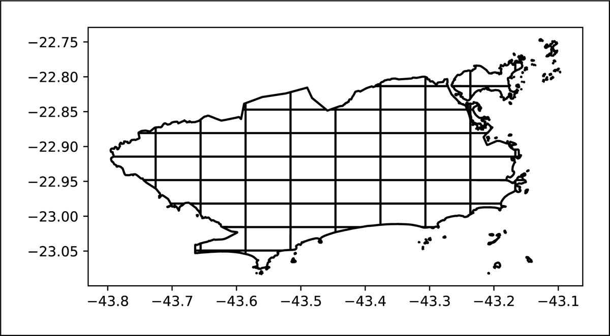
Figure 1
Space discretization of a region containing the city of Rio de Janeiro into rectangles, 76 of which have nonempty intersection with the region and are shown in the figure.
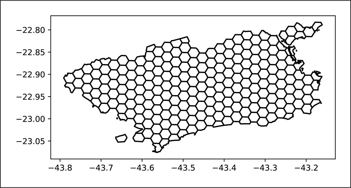
Figure 2
Space discretization of a region containing the city of Rio de Janeiro into hexagons using the Uber library H3 with scale parameter equal to 7.
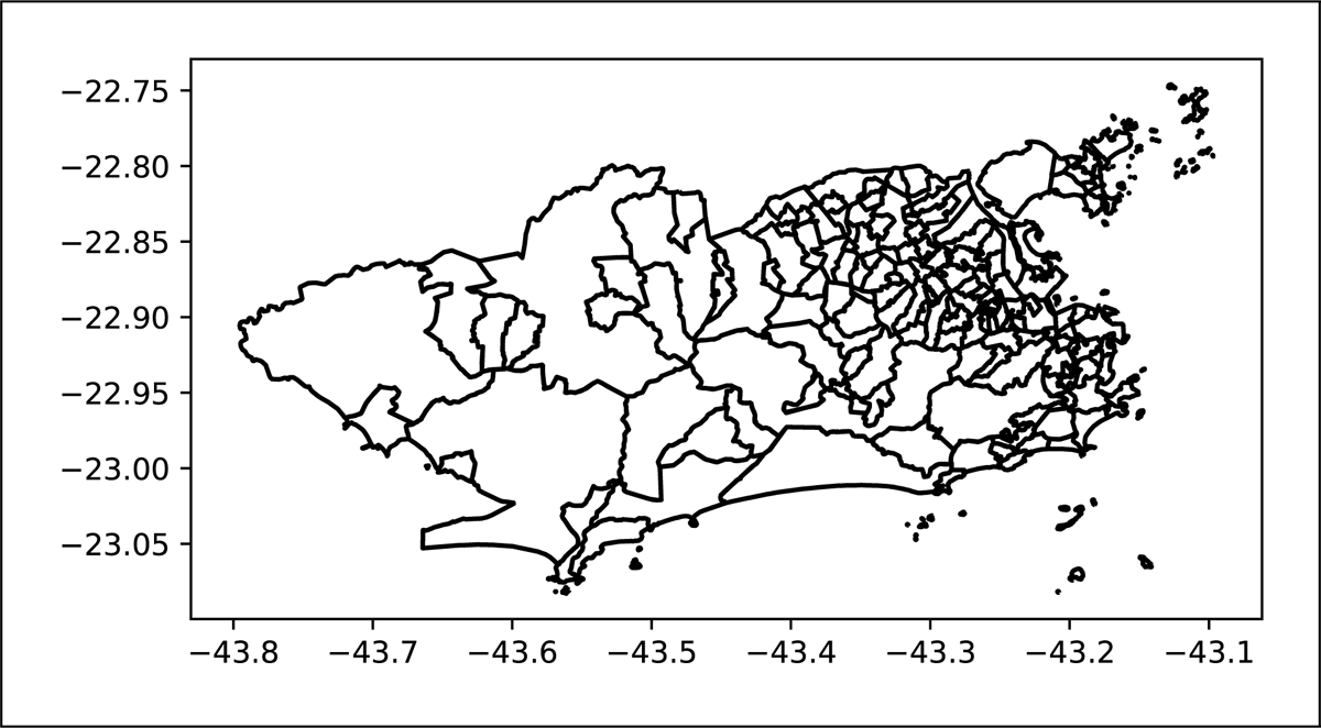
Figure 3
Space discretization of a region containing the city of Rio de Janeiro into 160 administrative districts.
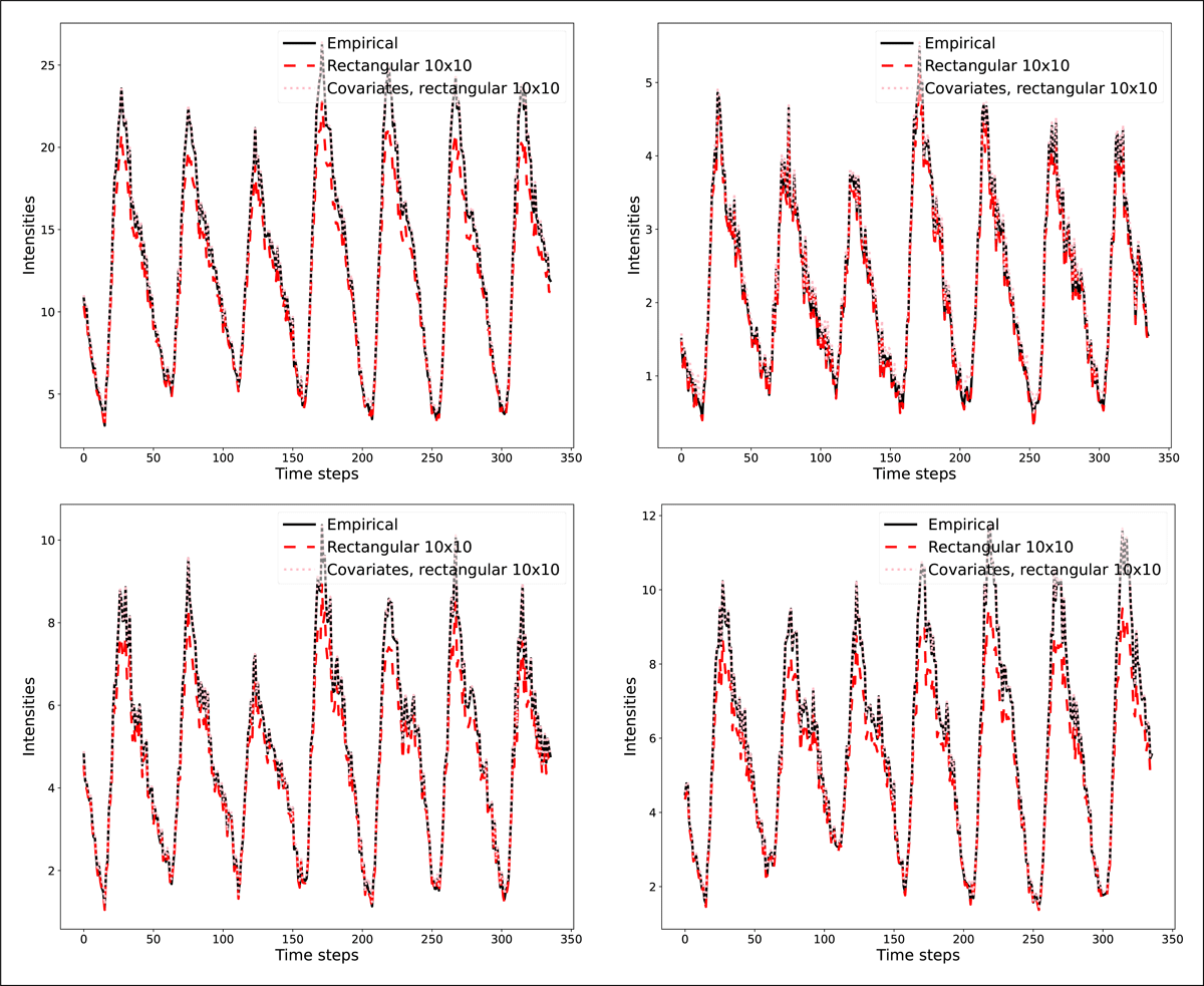
Figure 4
Aggregated estimates of the intensities for 3 estimators: (i) Empirical: the empirical intensities, (ii) Rectangular : Model M1 with the rectangular space discretization, and (iii) Covariates, rectangular : Model M2 with the rectangular space discretization. Top left: emergencies of all priorities, top right: high-priority emergencies, bottom left: intermediate priority emergencies, bottom right: low-priority emergencies.
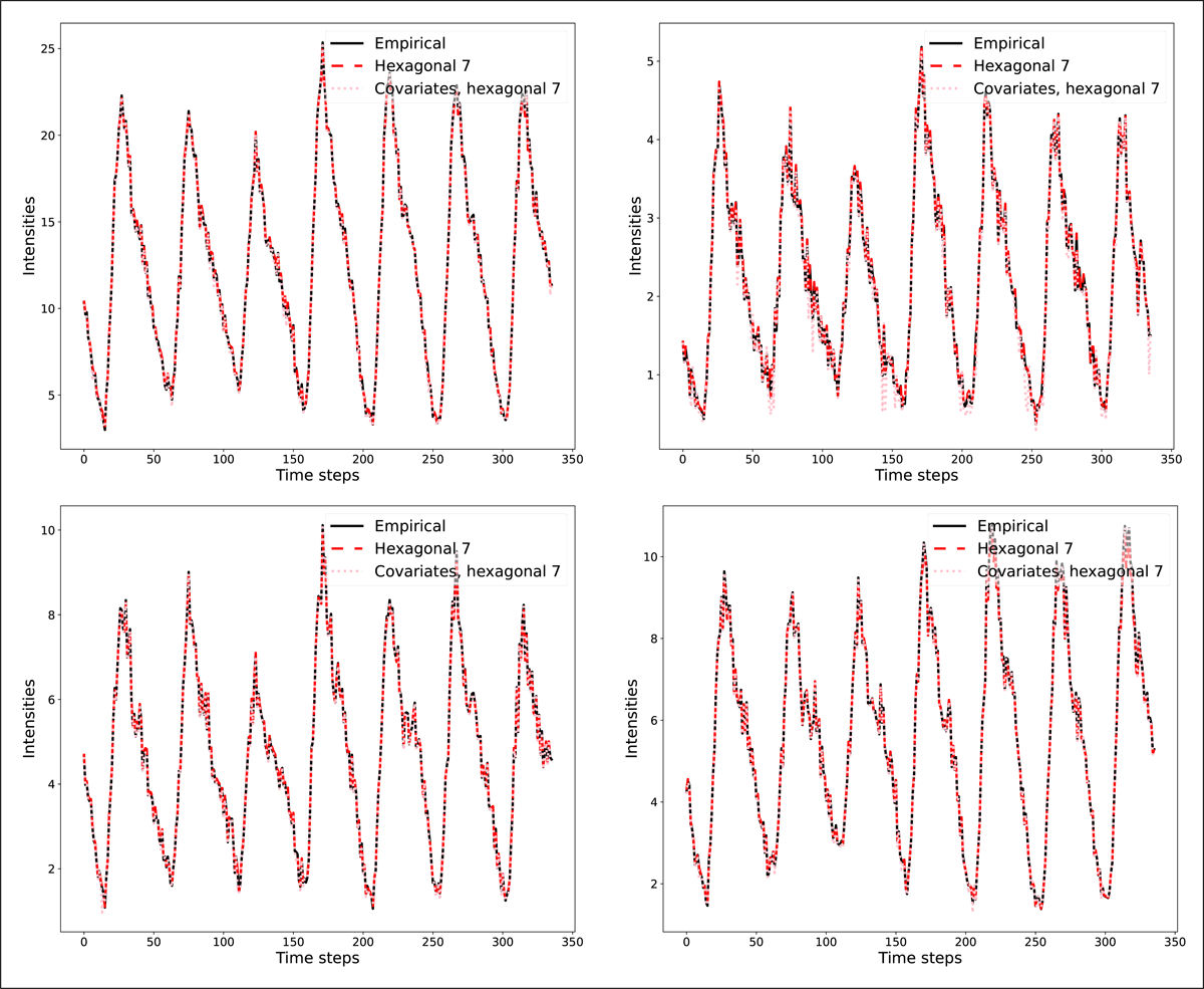
Figure 5
Aggregated estimates of the intensities for 3 estimators: (i) Empirical: the empirical intensities, (ii) Hexagonal 7: Model M1 with hexagonal discretization with scale parameter 7, and (iii) Covariates, hexagonal 7: Model M2 with hexagonal discretization with scale parameter 7. Top left: emergencies of all priorities, top right: high-priority emergencies, bottom left: intermediate priority emergencies, bottom right: low-priority emergencies.
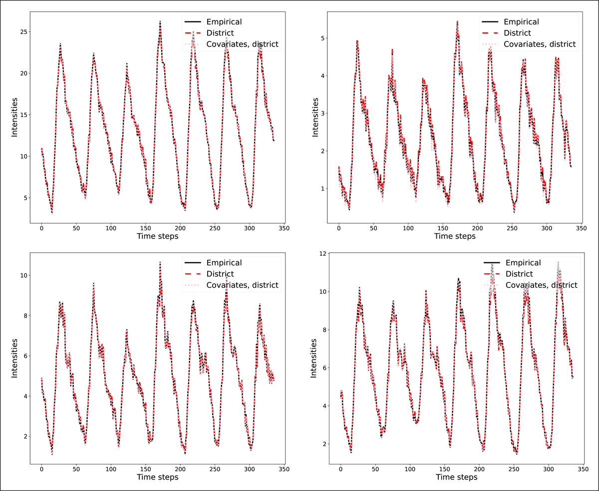
Figure 6
Aggregated estimates of the intensities for 3 estimators: (i) Empirical: the empirical intensities, (ii) District: Model M1 with the space discretization by districts, (iii) Covariates, district: Model M2 with the space discretization by districts. Top left: emergencies of all priorities, top right: high-priority emergencies, bottom left: intermediate priority emergencies, bottom right: low-priority emergencies.
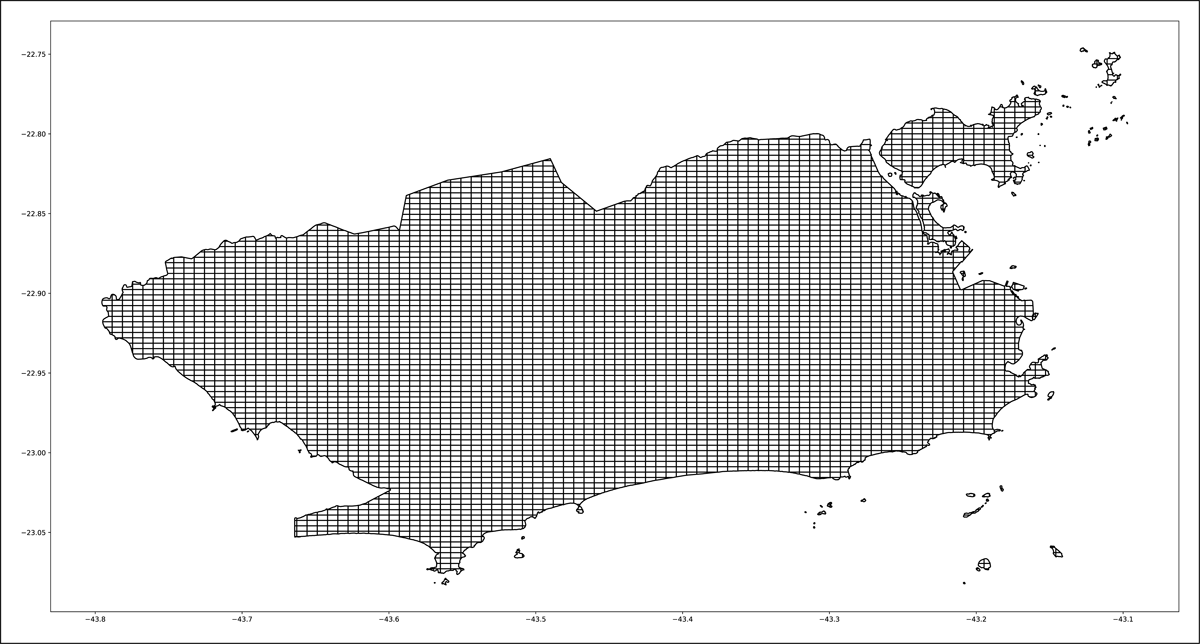
Figure 7
Space discretization of a region containing the city of Rio de Janeiro into rectangles, 4916 of which have nonempty intersection with the region and are shown in the figure.
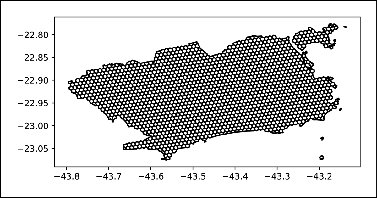
Figure 8
Space discretization of a region containing the city of Rio de Janeiro into hexagons using the Uber library H3 with scale parameter equal to 8.
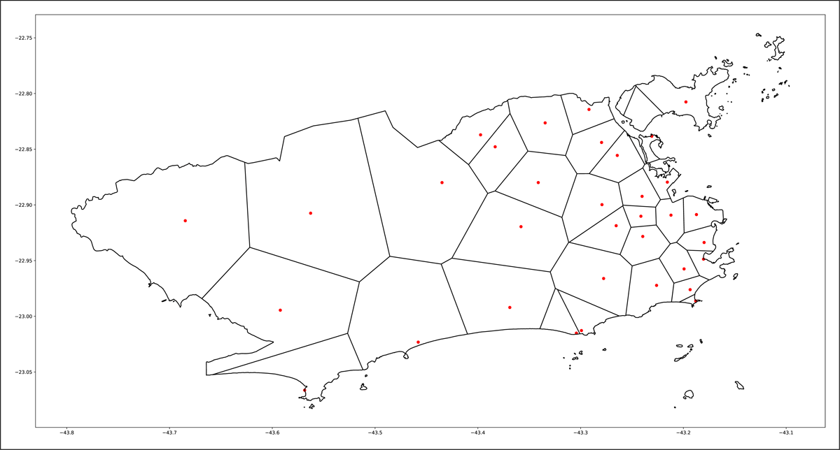
Figure 9
Discretization of a region containing the city of Rio de Janeiro into 34 subregions, given by the Voronoi diagram of ambulance stations in Rio de Janeiro.
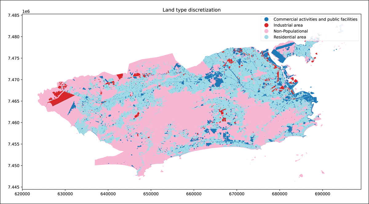
Figure 10
4 types of land use in Rio de Janeiro.
Table 2
Mean relative error . In column 1, m/n denotes for non-holiday time periods t, and for holiday time periods t.
| SAMPLE SIZE Ni,t | HOLIDAY | COV | NO COV 1 | NO COV 2 | NO COV 3 | EMP |
|---|---|---|---|---|---|---|
| 52 | 0 | 0.006 | 0.012 | 0.048 | 0.048 | 0.048 |
| 520 | 0 | 0.002 | 0.004 | 0.015 | 0.015 | 0.015 |
| 780 | 0 | 0.001 | 0.003 | 0.012 | 0.012 | 0.012 |
| 51/1 | 1 | 0.067 | 0.063 | 0.138 | 0.138 | 0.154 |
| 510/10 | 1 | 0.027 | 0.050 | 0.065 | 0.065 | 0.049 |
| 765/15 | 1 | 0.018 | 0.038 | 0.054 | 0.054 | 0.040 |
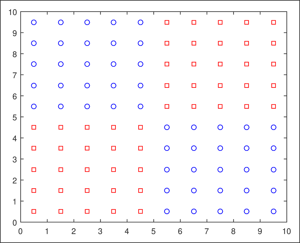
Figure 11
Test region . The intensity function is different in the blue and red subregions, but the user does not know about these subregions. For estimation purposes, the user discretizes into square zones.
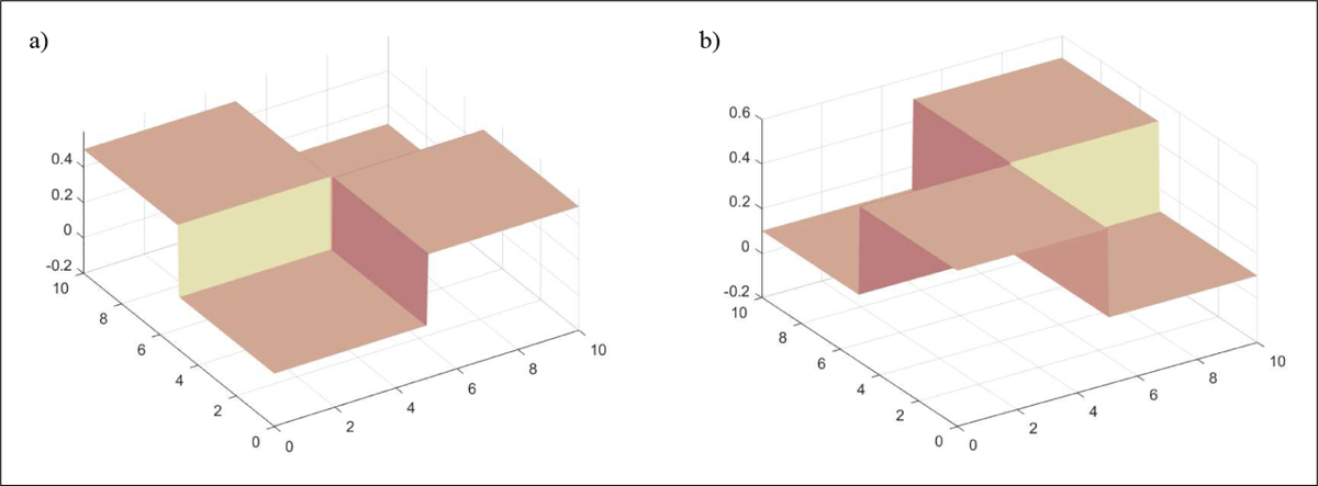
Figure 12
Intensities as a function of location, for time intervals that start at odd times and even times. (a) Time intervals that start at odd times. (b) Time intervals that start at even times.
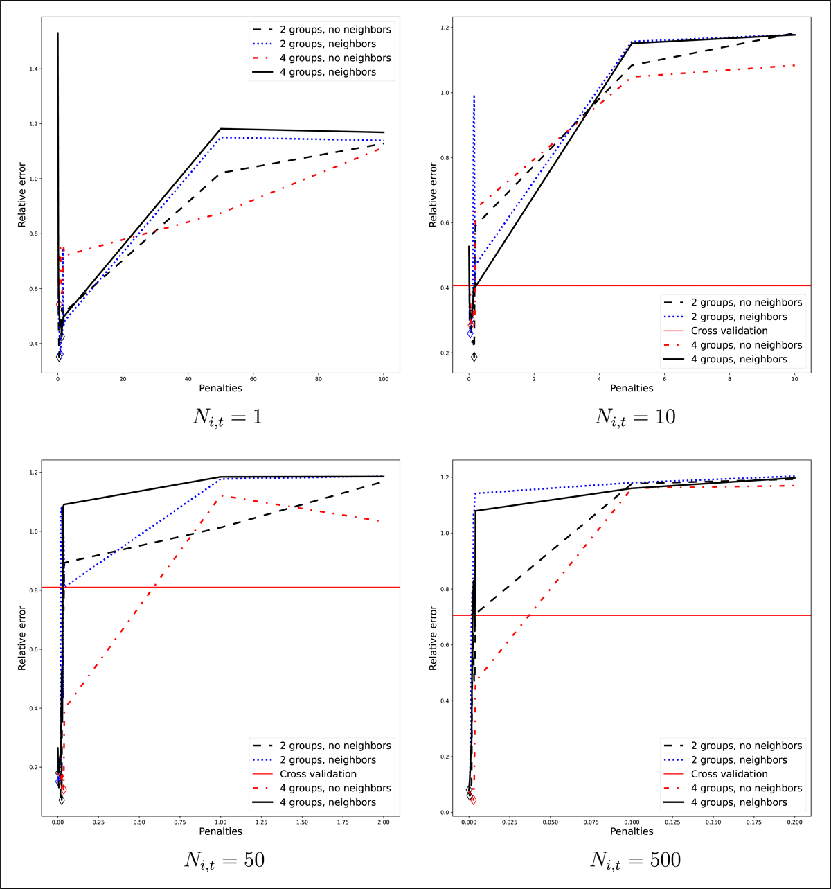
Figure 13
Mean relative estimation errors as a function of the penalty parameter w, for four sample sizes and six estimators (including the empirical estimator at ).
Table 1
The column headings denote the estimators as follows: Reg 1: estimator with partition of time intervals and with neighbor-based spatial regularization; Reg 2: estimator with partition of time intervals and without spatial regularization; Reg 3: estimator with partition of time intervals and with neighbor-based spatial regularization; Reg 4: estimator with partition of time intervals and without spatial regularization; CV: cross validation; Emp: empirical estimator. For each sample size and for each estimator Reg 1, Reg 2, Reg 3, Reg 4, each cell of the table gives two numbers separated by a slash (/): the first number is the minimum mean relative error over different values of penalty parameter w, and the second number is the value of w that attains the minimum. For the cross validation estimator, the first number is the mean relative error using the penalty parameter , and the second number is the value of . For the empirical estimator, the first number is the mean relative error using the penalty parameter .
| SAMPLE SIZE Ni,t | REG 1 | REG 2 | REG 3 | REG 4 | CV | EMP |
|---|---|---|---|---|---|---|
| 1 | 0.47/1.2 | 0.67/2.0 | 0.34/0.6 | 0.51/1.4 | - | 1.539/0 |
| 10 | 0.31/0.06 | 0.30/0.2 | 0.26/0.06 | 0.17/0.2 | 0.42/0.2 | 0.543/0 |
| 50 | 0.18/0.008 | 0.12/0.04 | 0.15/0.004 | 0.08/0.036 | 0.37/0.04 | 0.256/0 |
| 500 | 0.08/0.0 | 0.03/0.004 | 0.08/0.0 | 0.02/0.0028 | 0.26/0.002 | 0.07687/0 |
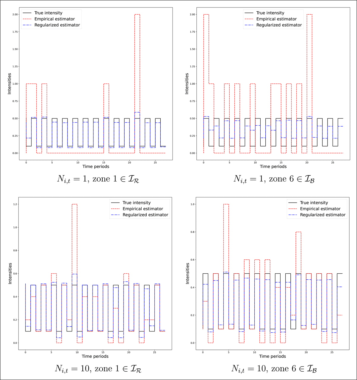
Figure 14
Comparison of true, empirical, and regularized estimates of the Poisson process intensities. True intensities as shown in Figure 12.
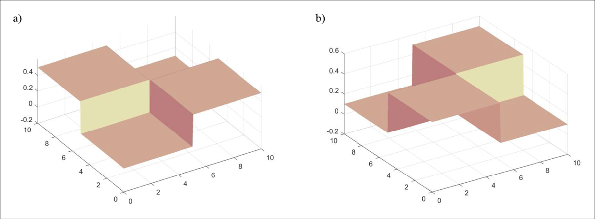
Figure 15
Intensities as a function of location, for time intervals that start at odd times and even times. (a) Time intervals that start at odd times. (b) Time intervals that start at even times.
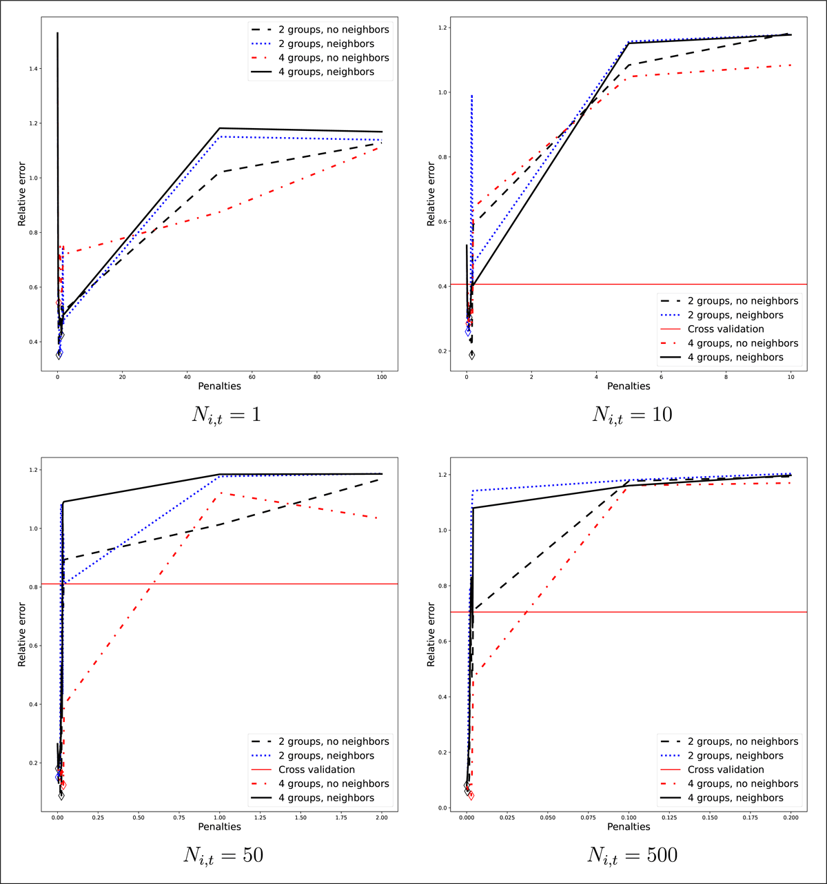
Figure 16
Mean relative errors as a function of the penalty parameter w. Intensities are as shown in Figure 15.
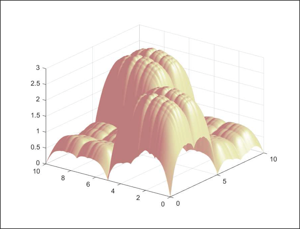
Figure 17
Graph of covariate function x1.