
(1) Overview
Introduction
In many applications, one has data of events that occur at points in space and time, and one wants to use the data to estimate spatio-temporal statistical models of the occurrence of such events. Examples of such spatio-temporal events are medical emergencies such as cardiac arrests, crimes such as robberies, earthquakes, weather events such as tornadoes, vehicles accidents, and fires. In these applications, one would like to use data to fit a function such as , where is a bounded subset of . Often, the domain is called “space” and the domain is called “time”. For example, may represent locations on a 2-dimensional map (in which case ), or locations in a 3-dimensional space (in which case ), or origin-destination pairs on a map (in which case ), and may represent time of the day (in which case hours), or time of the week (in which case hours). In this paper, we describe an open source software that uses spatio-temporal data to estimate a variety of statistical models that describe the spatio-temporal intensity f(x,t) of events of interest. We illustrate the use of the models and software using real data of medical emergencies.
A widely used nonparametric approach for fitting such a function f with data is to discretize space and time in a way that may depend on the data, and to fit a function from a chosen class on each discrete subset of the domain. There are many ways to construct such a discretization. Also, there are benefits to allowing the discretization to depend on the data. For example, a finer discretization may be chosen in regions of space and time with a higher concentration of data. There are also many function classes that can be used on each discrete subset of the domain. For example, the fitted function may be piecewise constant or piecewise linear, that is, it may be constant or linear on each discrete subset of the domain. Furthermore, sometimes one has data of covariates on the same space-time domain, with the covariates being correlated with the dependent variable. Even if the main purpose of the study is not to model the relation between the dependent variable and the covariates, these covariate data can be used in various ways to improve the estimates. For example, the covariates can be used in the choice of discretization by choosing the subsets of the discretization to be uniform in terms of the covariate values. The covariates can also be used as independent variables in a fitted parametric or semiparametric model. The covariates can also be used to regularize the model estimates, especially when the data are sparse.
Software tools for managing the choice of discretization, the regularization, and the model estimation, can be of great use. This paper describes such software tools for function estimation with spatio- temporal data.
Related Literature and Software
Spatio-temporal point processes consisting of data with a location and a timestamp arise in many applications such as the epicenters of earthquakes (1, 2), sudden crimes such as robberies and assaults (3), epidemiology (4, 5), and medical emergencies (6). For the theory of point processes, see (7, 8). (9, 10, 11, 12, 13, 14) provide overviews of statistical models and estimation for spatial and spatio-temporal point processes. (15) and (16) describe the use of R for processing spatial and spatio-temporal data and for model estimation. (17) describes the R package spacetime for converting spatio-temporal data among different formats, aggregating spatio-temporal data, and creating various types of plots.
The references above consider two types of models of the intensity function of a nonhomogeneous spatial or spatio-temporal Poisson process. One type of model is a nonparametric model such as the following. Let denote the observed points. A kernel function , and a smoothing parameter is chosen. Then the intensity model is given by
One challenge is that the effort to compute for a given x increases in the size N of the dataset. Another challenge is to select a good value for the smoothing parameter h. Several software packages make provision for the estimation of such kernel-based intensity models, including splancs (18) and spatstat (19). In contrast, LASPATED makes provision for the estimation of nonparametric models based on discretization of X. For example, let denote a partition of X. Then the intensity model is given by
where , , is estimated with data. LASPATED facilitates both the discretization as well as the parameter estimation.
Another type of model is a parametric model such as the following. Let , , denote a chosen collection of covariate functions, and let , , denote corresponding parameters to be estimated. Then the intensity model is given by
An advantage of the on the right side is that for all and all x. A disadvantage is that grows much faster when its argument is large than when its argument is small, which often results in poor fit and numerical instability. In contrast, LASPATED makes provision for the estimation of constrained parametric models such as
where typically z(X) is bounded. Several software packages make provision for the estimation of parametric intensity models of the form (3), including spatstat (19) and NHPoisson (20). More specifically, NHPoisson is an R package for the estimation and testing of parametric intensity functions of the form in one dimension, say time t. It is assumed that the covariate values are piecewise constant over integer intervals, that is, z(t) is constant for all for integers k. NHPoisson can use two optimization routines, optim and nlminb, to compute the maximum likelihood estimates of . NHPoisson also computes the inverse of the negative of the Hessian of the log-likelihood function as an asymptotic estimate of the covariance matrix of . NHPoisson computes the residuals and correlation metrics such as the Pearson correlation coefficient, and performs distribution tests such as the Kolmogorov-Smirnov test. (20) also specifically consider Poisson process approximations of peak over threshold models.
(21) proposed hybrid point process models with densities given by the normalized product of densities of a number of point processes, and described the use of spatstat for statistical inference for the hybrid models.
(22) describes the ppstat-package for analyzing data from multivariate point processes in time or one-dimensional space based on a specification of the conditional intensity process.
Application
Next, we describe the application that motivated the development of these software tools, and we demonstrate the use of these tools for the application. Phone calls about medical emergencies arrive at an emergency medical service (EMS) call center. Each emergency is characterized by a type, a location, and the arrival time of the call. The type of emergency is determined by the classification system used by the EMS, such as the Medical Priority Dispatch System (MPDS) or the Association of Public-Safety Communications Officials (APCO) system. Typical classification systems classify emergencies by the anatomical region (e.g., chest) affected, the cause of the emergency (e.g., animal bites), the importance of response time (e.g., “hot” versus “cold”), and the level of emergency service needed (e.g., basic life support versus advanced life support). The location is typically specified by an address, but can be converted to a latitude-longitude coordinate. The arrival time of the call is specified by a date-time combination.
We would like to estimate the arrival rate of emergencies as a function of emergency type, location, and time. Such an arrival rate function can be used to optimize the types and number of ambulances needed, the types and number of crew members needed, the crew schedules, and the positioning and dispatch of ambulances, and to develop a simulation of the emergency response system. We consider methods that discretize space and time and then estimate the arrival rate as a function of discrete space and time. While working on such a project (see 23, 24), we identified the lack of easy-to-use tools for this type of statistical work. Thus, the LASPATED library was created as a general tool to fill this gap. Then LASPATED was used with data of medical emergencies reported to the Rio de Janeiro EMS to fit arrival intensity functions. The data included the date and time of the phone call, the location of the emergency, and the type of the emergency. The emergency type data included a “priority level”: high, intermediate, and low-priority emergencies.
Different models of arrival intensity as a function of emergency type c, location i, and time t, were calibrated. The models were periodic with a period of one week. The time of the week was discretized into time intervals of length 30 minutes (thus the model had time intervals). Three different space discretizations are demonstrated:
A space discretization of a rectangle containing the city of Rio de Janeiro, shown in Figure 1 (76 of these rectangles have nonempty intersection with the city and are shown in the figure);
A hexagonal discretization of the city of Rio de Janeiro (obtained with scale parameter 7, with 297 hexagons intersecting Rio de Janeiro) shown in Figure 2;
A discretization by administrative districts of the city of Rio de Janeiro (with 160 subregions), shown in Figure 3.
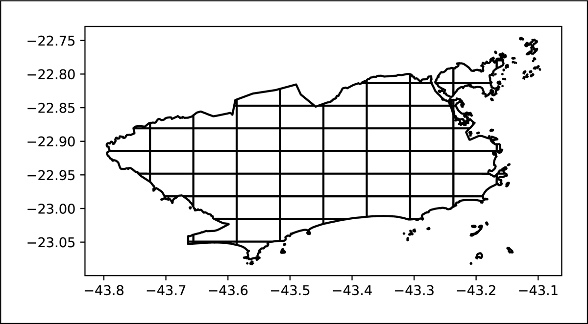
Figure 1
Space discretization of a region containing the city of Rio de Janeiro into rectangles, 76 of which have nonempty intersection with the region and are shown in the figure.
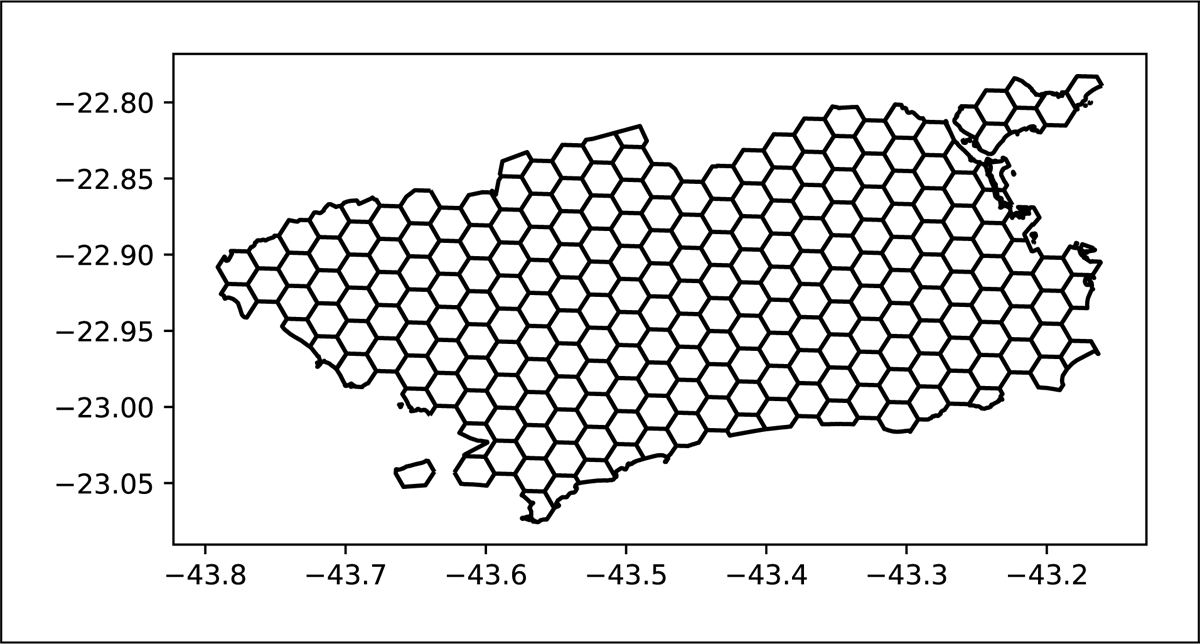
Figure 2
Space discretization of a region containing the city of Rio de Janeiro into hexagons using the Uber library H3 with scale parameter equal to 7.
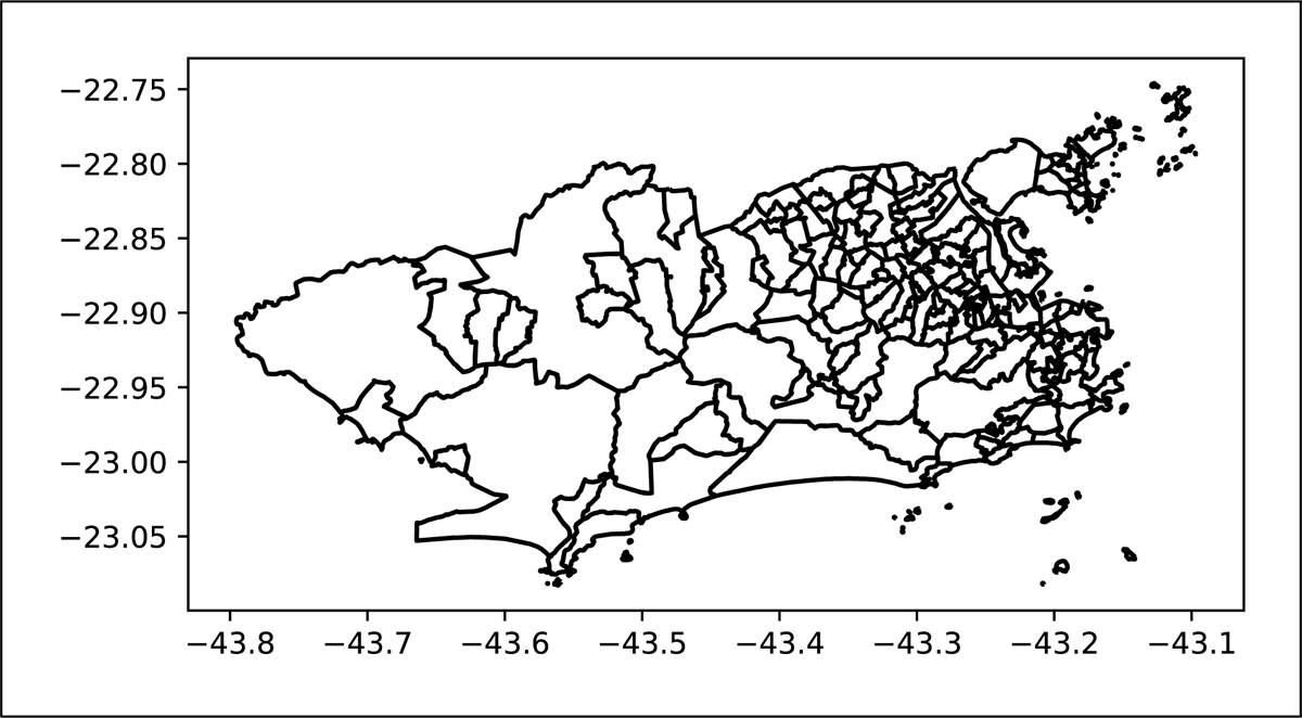
Figure 3
Space discretization of a region containing the city of Rio de Janeiro into 160 administrative districts.
For each space discretization, the model without covariates described in Section 2.1 (called Model M1 in what follows), and the model with covariates described in Section 2.2 (called Model M2 in what follows), were calibrated with LASPATED. For Model M2, we used the following four covariates: (a) the population of the zone, (b) the land area of commercial activities and public facilities in the zone, (c) the land area of industrial activities in the zone, and (d) the non-populated land area (such as forests, beaches, and water) in the zone. For the calibration of Model M1, we used regularization (see Section 2.1) with regularization parameter if zones i and j are neighbors, that is, if zones i and j share an edge or a vertex, and otherwise. The best value for w was selected from using cross validation. We did not regularize by time groups. The optimization problems for calibration were solved using the projected gradient method with Armijo line search along a feasible direction (see Section 2.3).
Figure 4 shows the aggregated estimated intensities using the rectangular discretization. More specifically, the top left plot of Figure 4 shows as a function of t, the top right plot of Figure 4 shows where c2 denotes the high-priority emergencies, the bottom left plot of Figure 4 shows where c1 denotes the intermediate priority emergencies, and the bottom right plot of Figure 4 shows where c0 denotes the low-priority emergencies. The intensity estimates shown in this figure are obtained with (i) the empirical mean number of calls for each call type, zone, and time interval, (ii) Model M1 with the rectangular space discretization, and (iv) Model M2 with the rectangular space discretization. In this example, all estimators give similar estimates of the aggregated intensities.
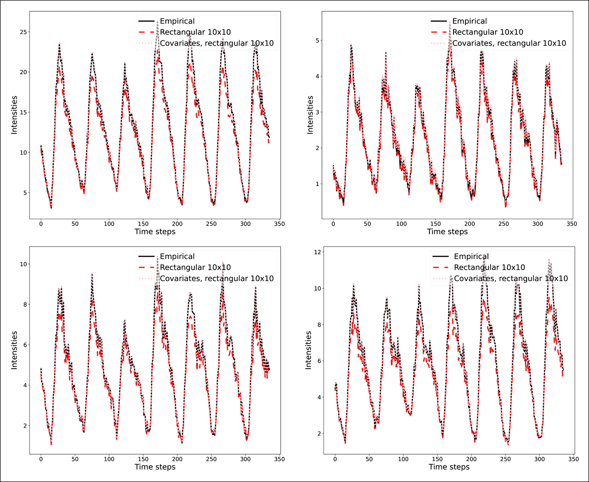
Figure 4
Aggregated estimates of the intensities for 3 estimators: (i) Empirical: the empirical intensities, (ii) Rectangular : Model M1 with the rectangular space discretization, and (iii) Covariates, rectangular : Model M2 with the rectangular space discretization. Top left: emergencies of all priorities, top right: high-priority emergencies, bottom left: intermediate priority emergencies, bottom right: low-priority emergencies.
Figure 5 shows the aggregated estimated intensities using hexagonal discretization with scale parameter 7. The top left plot of Figure 5 shows , the top right plot of Figure 5 shows , the bottom left plot of Figure 5 shows , and the bottom right plot of Figure 5 shows . The intensity estimates shown in this figure are obtained with (i) the empirical mean number of calls for each call type, zone, and time interval, (ii) Model M1 with hexagonal discretization with scale parameter 7, and (iii) Model M2 with hexagonal discretization with scale parameter 7.
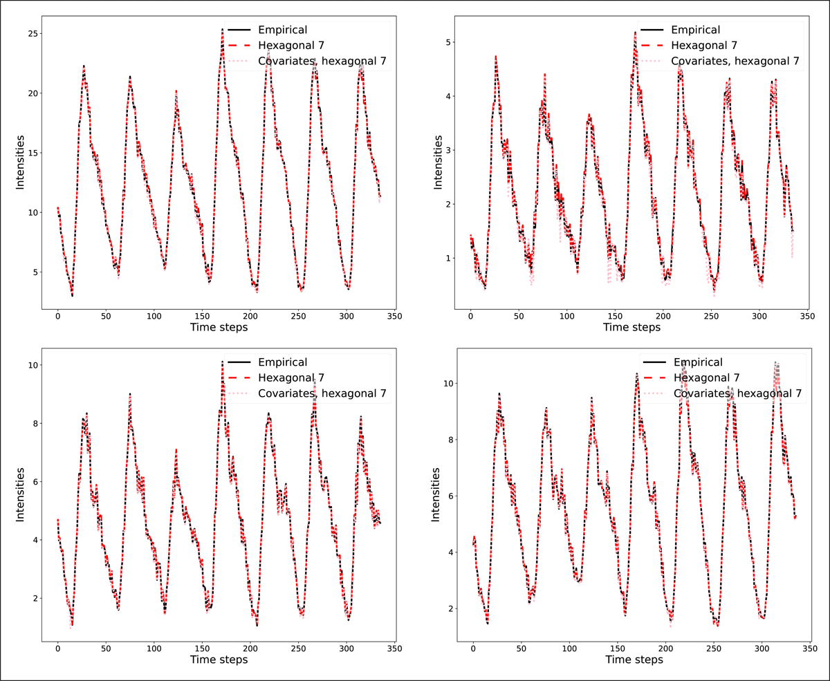
Figure 5
Aggregated estimates of the intensities for 3 estimators: (i) Empirical: the empirical intensities, (ii) Hexagonal 7: Model M1 with hexagonal discretization with scale parameter 7, and (iii) Covariates, hexagonal 7: Model M2 with hexagonal discretization with scale parameter 7. Top left: emergencies of all priorities, top right: high-priority emergencies, bottom left: intermediate priority emergencies, bottom right: low-priority emergencies.
Figure 6 shows the aggregated estimated intensities using discretization by district. The top left plot of Figure 6 shows , the top right plot of Figure 6 shows , the bottom left plot of Figure 6 shows , and the bottom right plot of Figure 6 shows . The intensity estimates shown in this figure are obtained with (i) the empirical number of calls for each call type, zone, and time interval, (ii) Model M1 with the space discretization by districts, and (iii) Model M2 with the space discretization by districts.
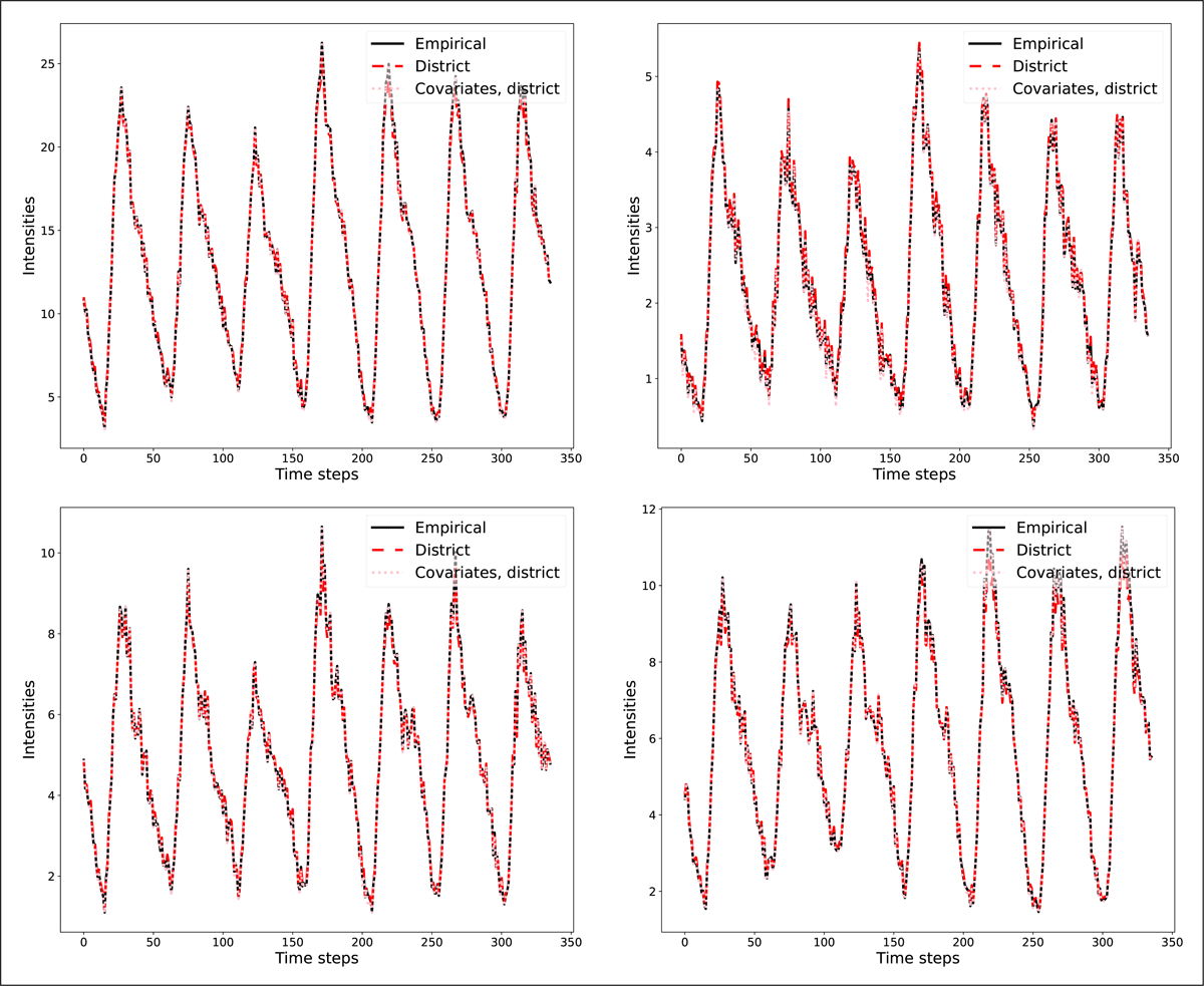
Figure 6
Aggregated estimates of the intensities for 3 estimators: (i) Empirical: the empirical intensities, (ii) District: Model M1 with the space discretization by districts, (iii) Covariates, district: Model M2 with the space discretization by districts. Top left: emergencies of all priorities, top right: high-priority emergencies, bottom left: intermediate priority emergencies, bottom right: low-priority emergencies.
Overview of the LASPATED Library
Various discretization methods to partition space and time were implemented in LASPATED, summarized next. LASPATED provides four types of space discretization: in rectangles, in hexagons, based on the Voronoi diagram/Dirichlet tessellation for a set of points in , and customized discretizations. LASPATED also provides functions to combine information from two different space discretizations, such as functions to calculate the areas of intersection of pairs of subregions from two discretizations, or to calculate location data such as population in the intersection of pairs of subregions from two discretizations.
LASPATED also provides various types of time discretization. For example, a simple partitioning of time could be a partition of the week in time intervals of 1 hour each. Then the corresponding time intervals are
Time intervals of different types can also be distinguished. For example, there could be different time intervals such as Monday [0:00,1:00) for different holidays, or there could be different time intervals such as Friday [20:00,21:00) depending on the scheduling of a sport event at the time. For instance, for the time window Friday [20:30,21:00), one could have
a time interval for Friday [20:30,21:00) on days which are holidays and a major sport event is scheduled;
a time interval for Friday [20:30,21:00) on days which are holidays and a major sport event is not scheduled;
a time interval for Friday [20:30,21:00) on days which are not holidays and a major sport event is scheduled; and
a time interval for Friday [20:30,21:00) on days which are not holidays and a major sport event is not scheduled.
Given a point in space and time , possibly with additional characteristics such as holiday or event type, LASPATED determines the combination of spatial subregion and time interval for the chosen discretization that contains the given point . Furthermore, given a data set of observations consisting of several points, LASPATED computes the number of points in the data set in each combination of spatial subregion and time interval for the chosen discretization. For example, given a data set of medical emergencies, with a week of data associated with each observation, LASPATED computes the number of emergencies in the data set for each combination of type of emergency, spatial subregion, and time interval, for the chosen discretization, for each week of data.
LASPATED also facilitates calibration of nonhomogeneous spatio-temporal Poisson models using data prepared with the discretization subroutines. For example, suppose that the number of points of a spatio-temporal Poisson process is a function of type, spatial location, and time, and that a piecewise constant arrival rate model for type c, spatial subregion i, and time interval t, is estimated. LASPATED provides two approaches discussed in Section 2 to calibrate such models. Both approaches allow one to estimate with sparse data, for example when there are many combinations of subregion and time window in the discretization relative to the amount of data. In the first approach, the intensities are the solutions of an optimization problem which optimizes a linear combination of the log-likelihood and a regularization term that may include covariates or penalize non-smoothness of intensities regarding space and time. In the second approach, covariates are used as auxiliary explanatory variables in the model.
To the best of our knowledge, LASPATED is the first software that:
implements the calibration of the models we propose for spatio-temporal data;
provides a complete analysis and calibration of statistical models for spatio-temporal data taking only historical data as inputs and providing as outputs a discretized process, Poisson intensities, and scenarios for future arrivals;
offers such a large set of options for spatial discretization;
offers such a large set of options for time discretization;
handles arrival types for discretization and provides outputs using information from several discretizations of several types of data.
Implementation and Architecture
1 Overview of Implementation and Functionalities
LASPATED contains a Python module that handles space and time discretization functions, given a dataset of events, and a C++ module that performs model estimation from the discretized set of events. The Python module is available on Pypi (Python package index) while the C++ source code is available on GitHub. Additionally, we provide an application for the model estimation tool for users unfamiliar with C++. The app may be used via a Docker image.
Python LASPATED module uses popular data science modules like (geo)pandas, shapely, numpy and matplotlib to perform its tasks. The user must provide a csv file, with header columns, containing data of events, see our user manual for details. Our spatiotemporal events in this file are identified by at least three columns: latitude, longitude, and a timestamp. If the events have other features, the user may provide a list of columns containing such features.
The border of the studied region may be defined from a Shapefile provided by the user, or LASPATED may obtain it from the events, defining a rectangle or a convex hull of the data that contains all events.
Space discretization may be done in four formats: rectangular, hexagonal, customized by regions, or using a Voronoi diagram for a set of locations. The hexagonal discretization is done via Uber python package H3. To use the customized discretization (for instance, administrative districts of a city), the user must provide a geopandas dataframe containing the subregions. The Voronoi diagram is computed from a dataframe containing latitude/longitude pairs, for instance, the locations of police stations for crime data.
If there is other data available for the area containing the data, such as population or land type, LASPATED allows us to combine this information with the spatiotemporal events. For instance, if the user provides a geopandas dataframe contaning the population of a region, LASPATED is able to compute the population inside each discretized subregion.
LASPATED allows users to specify a rich diversity of time discretizations, see below.
At the end of the discretization process, LASPATED outputs two dataframes:
a geopandas dataframe containing data about space discretization, including the geometry of each subregion, its index, and attributes;
a dataframe including for each event its features, its spatial discretization index related to the geopandas dataframe, and its time discretization indices.
LASPATED allows users to save these dataframes to a file or as a plot. The discretized data can also be saved as aggregates by discretization indices.
The C++ module takes spatio-temporal discretized events data (possibly generated by the Python module) and uses a projected gradient algorithm to solve the maximum likelihood estimation problem.
Next, we describe the statistical models on which LASPATED is based.
2 Poisson Models with Discretized Spatio-temporal Data
In this section, we describe the models that motivated the work on LASPATED, and we explain how LASPATED solves the optimization problems for the calibration of these models. We will use the medical emergency application as a running example to explain the models.
Let index the subsets of the space discretization forming a partition of the region ; the elements of will be called zones. Let index the subsets of the time discretization forming a partition of all times of interest; the elements of will be called time intervals. Let denote the set of point types; can be any finite set that forms a partition of all space-time points of interest; the elements of will be called types.
2.1 Model without Covariates
Each time interval has a duration (in time units). It is assumed that data are observed for multiple occurrences of the same interval t, and that each time data are observed for a type , zone , and interval , all such space-time points in the same time interval are recorded in the data. For example, suppose that forms a partition of the week in time intervals of 1 hour each. Then it is assumed that the data contain observations of emergencies of type c in zone i during hour t for multiple weeks, and that each time emergency arrivals of type c in zone i are observed during a particular hour t of a particular week, all the emergency arrivals of the same type in the same zone during the same hour t of that week are recorded. (It is planned to make provision for censored data in future work.) All the emergency arrivals of a particular type c in a particular zone i during a particular hour t of a week together are called an observation. For each , , and , let Nc,i,t denote the number of observations for type c, zone i, and time interval t, and let these observations be indexed by . For each , , , and , let Mc,i,t,n denote the number of points (arrivals) for observation n of type c, zone i, and time interval t, and let denote the total number of points over all observations for type c, zone i, and time interval t.
Assume that are independent (but not necessarily identical) Poisson distributed random variables. Let denote the mean number of points per length of time (such as per hour) for type c, zone i, and time interval t. Then random variable Mc,i,t,n is Poisson distributed with mean . Let . Then the likelihood function is
and intensities that maximize the log-likelihood are the same intensities that solve
A typical issue with such applications is that the distribution of data is far from uniform — there are a few combinations of type c, zone i, and time interval t with many observations, but for most combinations of type c, zone i, and time interval t there are very few observations. In such cases, it may be advantageous to use data from “neighboring” observations, or to bring additional data to bear on the estimation problem.
For example, suppose that forms a partition of the week in time intervals of 1 hour each, but that it is expected that many hours of the week are similar to other hours of the week in terms of arrival rates. A simple approach to incorporate such an idea is to partition into a collection of subsets of in such a way that it may be reasonable to expect that, for each , , and , the values of for different will be close to each other (but not necessarily the same). Let denote a similarity weight for . Another approach to incorporate such an idea is to specify a similarity weight for each (unordered) pair . For example, if t and t’ are neighboring time intervals, and otherwise. Similarly, it may be expected that many zones are similar to other zones in terms of arrival rates. Such an idea can also be incorporated by partitioning the set of zones into subsets, each with its own similarity weight, or by specifying for each pair , a similarity weight . An example loss function with similarity regularization that uses the first approach for time intervals and the second approach for zones is given by
Example 2.1: Consider a simple example in which , and and are singletons, that is, is estimated as a function of space only. Suppose that the number of observations is the same for all . Note that the empirical estimates, without smoothing, are . For smoothing, choose for all , and otherwise, that is, zone 0 is a neighbor of all other zones, but none of the other zones are neighbors of each other. Then the loss function in (6) reduces to
It follows from the first-order optimality conditions that
Unless for all i, it follows from that , that is, the estimated total rate is biased low.
To counter the bias illustrated in Example 2.1, one may want to use the data to constrain the estimates . For example, taking duration of time interval t into account, one may want to constrain the estimates so that for every type , the sum of the intensities is equal to the sum of the empirical intensities over zones and time intervals . The corresponding constraint is
Intensity estimates are then obtained by solving
2.2 Model with Covariates
Each type c, zone i, and time interval t may have covariates that are correlated with the arrival rates , and data of these covariates can be used to partly compensate for sparse data. For example, emergency arrival rates in different zones and time intervals can be expected to be correlated with the population and other measures of economic activity in the zones, as well as with festivals and other events during the time intervals. For each , , and , let denote the covariate values of type c, zone i, and time interval t. For example, may be the population count with home addresses in a zone i, and may be an indicator that a major sports event is scheduled in a zone i during a time interval t. Then consider the model
where are the model parameters. Let denote the set of all possible values of xc,i,t. Often can be chosen to be a polyhedron. Note that it should hold that
To facilitate such a model, let denote the total number of observations, and let these observations be indexed . For each observation , let Mn denote the number of arrival points for observation n and let denote the covariate values of observation n. Then the negative log-likelihood function is given by
As for the model without covariates, one may want to use the data to constrain the estimates . For example, one may add the constraint that for every type , the sum over all zones and all time intervals of the estimated rates is equal to the sum over all zones and all time intervals of the empirical rates, that is the constraint
Next, we provide two examples of such models.
Example 2.2: Index , , and let . For each , , and , let be the number of people resident (population count) in the zone of observation n if observation n is for type c and time interval t, and otherwise. The next covariate is a set of occupational land use areas (in km2), for instance the areas of commercial activities and public facilities, of industrial activities, and of undeveloped land. Index the occupational land uses by . For each , , , and , let be the area of occupational land use m in the zone of observation n if observation n is for type c and time interval t, and otherwise. Then denotes the forecasted number of arrivals for the type of observation n in the zone of observation n during the time interval of observation n due to people being in the residential area, which is modeled as proportional to the number of people resident in the zone of observation n with a proportionality coefficient that depends on the type and the time interval. Similarly, denotes the forecasted number of arrivals for the type of observation n in the zone of observation n during the time interval of observation n due to people being in the different occupational areas which is modeled as proportional to the areas of occupational land use in the zone of observation n with a proportionality coefficient that depends on the type and the time interval. If is large, the number of parameters of the model specified in this example is also large. Similar to (6), similarity regularization can be used to estimate the parameters, for example, by minimizing a loss function such as
Example 2.3: This example will be used to demonstrate the modeling of arrivals of emergency calls to an emergency medical service. The sets , , and are the same as in Example 2.2. Let denote the indices of discrete time periods during a day, for example, if each day is discretized into 30-minute intervals. Let denote the set of indices of the (normal) days of the week, as well as indices for special days such as holidays. Thus, the cardinality of is 7 plus the number of special days. A pair specifies a time interval. For each zone , consider covariates , where is the population count in zone i, and is the area (in km2) of occupational land use j in zone i for . Here, we assume that these data (population and land type areas) do not depend on time, which is reasonable for moderate time periods. Then, for each type c, zone i, day d, and time period t, the arrival intensity is given by for some vector ). Furthermore, for each type c, zone i, day d, and time period t, let Nc,i,d,t denote the number of observations, let Mc,i,d,t,n denote the number of arrival points for observation n, and let . Then the negative of the log-likelihood function is given by
Note that call rates should be positive. Additionally, for each type c, day d, and time period t, the coefficients that represent the ratio of emergencies to population should be small (say less than 1), which implies the constraints . Therefore, the estimation problem is to solve the optimization problem
Depending on the solver, better numerical performance may be obtained by replacing the constraints of (14) with
for some sufficiently small.
2.3 Solving the Optimization Problems
The calibration of models such as those of Section 2.1 requires solving an optimization problem (8) of the form . The problem can also be formulated as
where C is a closed convex set such as
for a chosen and e a vector of ones. The objective function of (16) is differentiable on such C.
The calibration of models such as those of Section 2.2 requires solving an optimization problem (14) of the form
where B is given by constraints such as (15). In both cases, the problem is a convex optimization problem with a differentiable objective function on the feasible set.
The algorithms described below for solving problems such as (16) take regularization weights such as WG and wi,j as input. LASPATED also provides cross validation functions, that facilitate use of the data to select regularization weights.
Projected gradient with line search. LASPATED provides the following two methods for solving problems (16) and (18): (1) a projected gradient method with line search along a feasible direction, and (2) a projected gradient method with line search along the boundary. These methods follow (25) except for the update of . Here, we provide the pseudocode for these methods for a problem of form (16). Let denote the projection of the point onto a closed convex set C. The pseudocode presents methods that are run for a chosen number of iterations and that start from any feasible . For alternative stopping criteria, see the discussion at the end of this section.
Projected gradient method with Armijo line search along a feasible direction for convex problem (16)
Initialization: Choose , , MaxNumberIteration , and an initial feasible point
, ,
While MaxNumberIteration
Compute and
zAux = z
Compute
While
Compute
End While
End While
Projected gradient method with Armijo line search along the boundary for convex problem (16)
Initialization: Choose , , MaxNumberIteration , and an initial feasible point
, ,
While MaxNumberIteration
Compute and
Compute
While
Compute
End While
End While
Note that for problem (16) with , the projection onto C is easy to compute, where the max is taken componentwise. Furthermore, the first derivatives of are given by
where G(t) denotes the group of time intervals to which t belongs. For problem (18), the first derivatives of are given by
For problem (18) with , the projection onto B is computed by solving a convex quadratic problem.
Stopping test for projected gradient method with line search. LASPATED makes provision for several stopping criteria such as convergence of the objective function values, a maximum number of iterations, or stopping when optimality conditions are approximately satisfied. We give more details about this latter criterion. Consider an optimization problem
where and C are convex, and C is compact. At the end of iteration k, points have been generated, and the upper bound
on can be computed. One can minimize the linear approximation of at to compute the lower bound
or one can minimize the piecewise linear approximation of at to compute the lower bound
The algorithm is stopped when
thus obtaining an -optimal solution.
3 Time Discretization
LASPATED provides multiple types of time discretization. The corresponding function is add_time_discretization — see the user manual for details of the use of this function to produce the time discretizations described below. Some time discretization methods are based on a periodic pattern. The duration of the periodic pattern can be chosen, for example, 7 days or 10 days or 3 months. To make provision for holidays and special events, LASPATED also facilitates time discretization methods that are not based on a periodic pattern. The subsets of the time discretization can be chosen to be time intervals, or finite unions of time intervals. For example, if the duration of the periodic pattern is 7 days, then Monday [08:00,09:00] Friday [17:00,18:00] can be chosen to be one subset of the time discretization. Next, we mention some special cases of time discretization facilitated by LASPATED.
3.1 Periodic with Equal Length Time Intervals
The simplest time discretization in LASPATED uses a periodic pattern, in which the duration of the periodic pattern is partitioned into time intervals of equal length. That is, each subset of the time discretization is a single time interval, and all these time intervals have the same length.
3.2 Periodic with Unequal Length Time Intervals
Another time discretization in LASPATED also uses a periodic pattern, in which the duration of the periodic pattern is also partitioned into time intervals, but the time intervals may have unequal lengths. As in the previous method, each subset of the time discretization is a single time interval, but unlike the previous method, all these time intervals do not have the same length.
3.3 Customized Subsets
LASPATED makes provision for customized subsets to facilitate holidays and special events. Each customized subset is assigned a unique index number, and consists of one or more time intervals. Each time interval is specified by its start time and its end time, as well as the index of the subset that the time interval belongs to. Time points that do not belong to any customized interval, belong to the customized subset with index 0. LASPATED also allows time intervals to repeat. For example, a time interval that starts and ends on date 2016-01-01 (New Year’s Day) may be specified to repeat each year. If the time interval is specified as repeating yearly, then for all observations on the same day of the year (such as January 1), the time intervals’ start time during the day, end time during the day, as well as the index of the subset that the time intervals belong to, will be the same for all years.
4 Space Discretization
LASPATED provides several space discretization tools. The corresponding functions are add_max_borders, plot_discretization, add_geo_discretization, get_intersection, add_geo_variable, get_events_aggregated, write_arrivals, write_regions — see the user manual for details of the use of this function to produce the space discretizations described below.
4.1 Defining Borders
The first step for space discretization is to choose a coordinate system and to specify the border of a region that contains the locations of all the points in the dataset. The border specifies the region that will be discretized in space. The border can be specified with LASPATED using different methods.
4.1.1 Custom Map
A custom map can be provided to LASPATED by specifying the coordinates of a sequence of vertices on the border of the region. Typically, a Shapefile is provided for this purpose; the user manual and the video tutorial contain details and examples.
4.1.2 Rectangular Border and Convex Hull
LASPATED can be instructed to determine various regions that contain the locations of all the points in a dataset, such as the smallest rectangle that contains all the points in the dataset, or the approximate convex hull of all the points in the dataset.
Once borders are specified, the space discretization step partitions the region inside the specified border into subregions. Similar to the subsets of the time discretization, the subregions of the space discretization can be chosen to be simple shapes such as rectangles or hexagons, or unions of simple shapes. Next we mention some special cases of space discretization facilitated by LASPATED.
4.2 Equal Sized Rectangular Space Discretization
The simplest space discretization in LASPATED partitions the region into equal sized rectangles, in such a way that adjacent rectangles share a common face, that is, if the boundaries of rectangle A and rectangle B intersect, then either rectangle A and rectangle B intersect in one (corner) vertex, or rectangle A and rectangle B share an edge between 2 vertices. For example, the rectangles and are adjacent but do not share a common face. If the region is not a union of these equal sized rectangles, then the intersections of the rectangles with the region may not be equal sized. For example, Figure 1 shows a discretization of a custom region containing the city of Rio de Janeiro into rectangles, and Figure 7 shows a discretization of the same region into rectangles. Both discretizations were obtained with LASPATED.
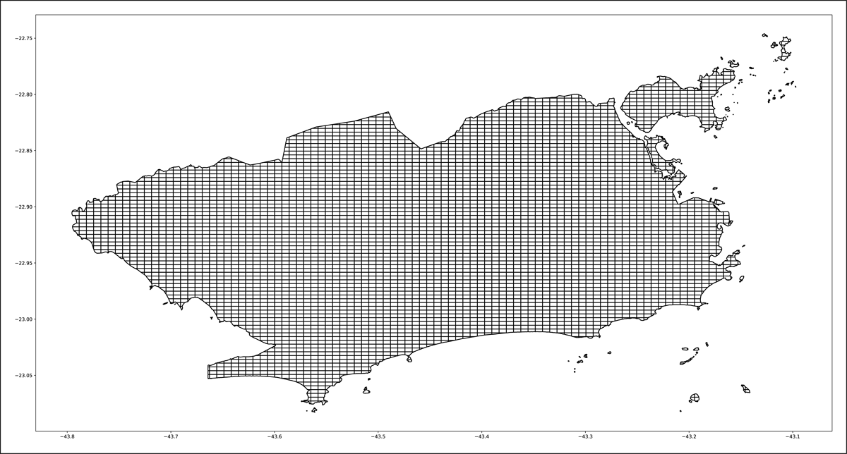
Figure 7
Space discretization of a region containing the city of Rio de Janeiro into rectangles, 4916 of which have nonempty intersection with the region and are shown in the figure.
4.3 Equal Sized Hexagonal Space Discretization
Another simple space discretization in LASPATED partitions the region into equal sized hexagons, in such a way that adjacent hexagons share a common edge. (The Uber Python package H3 was used for the discretization.) Figure 2 shows a discretization of a region containing the city of Rio de Janeiro into hexagons using a scale parameter equal to 7, and Figure 8 shows a discretization of the same region into hexagons using a scale parameter equal to 8. Both discretizations were obtained with LASPATED.
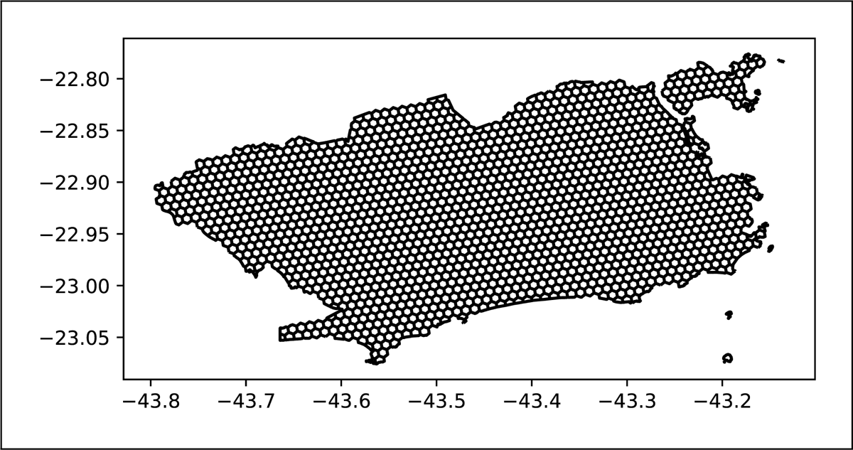
Figure 8
Space discretization of a region containing the city of Rio de Janeiro into hexagons using the Uber library H3 with scale parameter equal to 8.
4.4 Customized Space Discretization
LASPATED also facilitates space discretization with customized subregions. For example, Figure 3 obtained with LASPATED displays a customized discretization of the city of Rio de Janeiro into 160 administrative districts.
4.5 Discretization using Voronoi diagrams
LASPATED also provides space discretization with Voronoi diagrams. Figure 9 obtained with LASPATED displays a discretization based on the Voronoi diagram given by the locations of ambulance stations in Rio de Janeiro. Each subregion includes the set of points that are closest to a specific station.
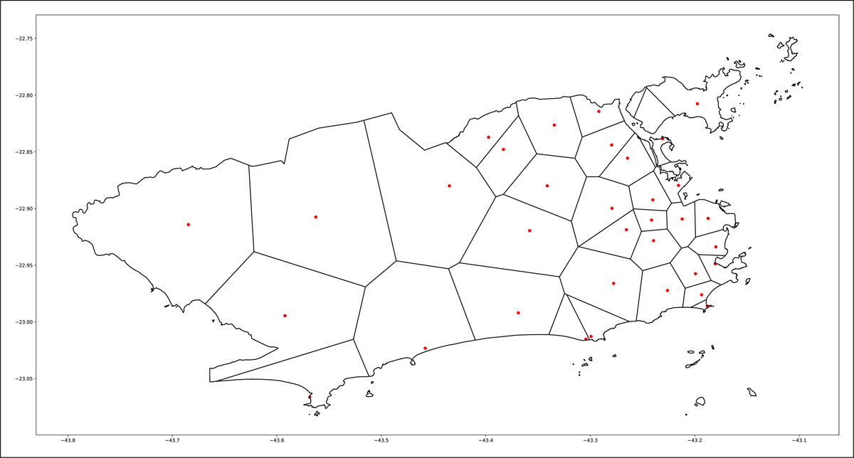
Figure 9
Discretization of a region containing the city of Rio de Janeiro into 34 subregions, given by the Voronoi diagram of ambulance stations in Rio de Janeiro.
5 Additional Discretization Functionalities
Often different discretizations are used for different purposes. For example, different spatial attribute data such as population count and land use type may be provided using different space discretizations. Consider two discretizations D1 and D2. Let be the index set of the subregions of discretization D1, and let be the index set of the subregions of discretization D2. In this context, LASPATED provides the following functionalities:
Given subregion indices and , LASPATED computes the area of the intersection of subregions i1 and i2. As an example, Figure 10 displays a partition of Rio de Janeiro into 4 different types of land use. LASPATED can be used to compute for every subregion of a given space discretization (such as rectangles or hexagons) the area of each land use type in the subregion.
Consider a given attribute, such as population count, and assume that the attribute value in each subregion of discretization D1 is uniformly distributed with density , where is the area of the subregion i1. We want to allocate this attribute value to the subregions of another discretization D2. LASPATED computes the value of the attribute allocated to subregion of discretization D2 as .
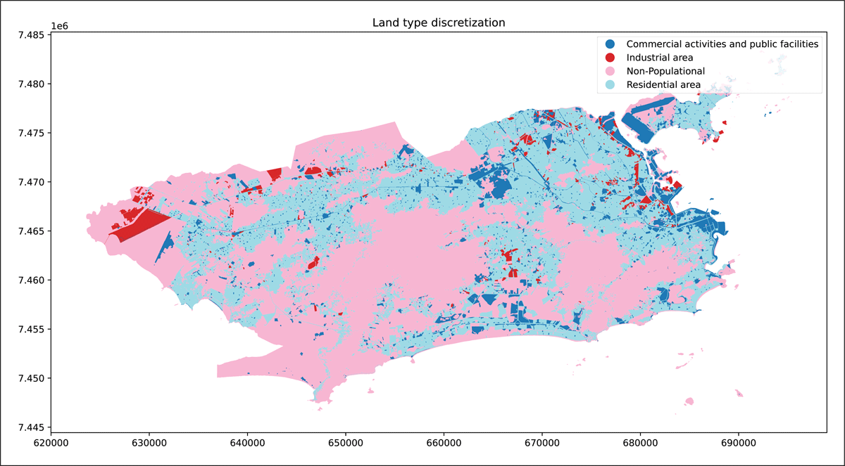
Figure 10
4 types of land use in Rio de Janeiro.
6 Calibration Functions
LASPATED also provides tools in C++ for the calibration of the models described above. All code is contained in the header file laspated.h. The user can run the calibration functions by building a model object and a struct with parameters for the projected gradient and cross validation functions (see the user manual for details) or by using the application we provide, as described in Section 6.2. The next section discusses the compilation and dependencies.
6.1 Compilation and Dependencies
C++ calibration functions use the following libraries:
Gurobi (https://www.gurobi.com), an optimization tooblox used only in the model with covariates;
xtensor and xtl libraries.
When compiling the code, the user needs to pass the location of the header files for LASPATED, xtl, xtensor and gurobi, as well as the location for Gurobi libraries and their respective flags. xtl and xtensor require the C++14 standard and its flag must also be passed. The example below compiles an executable called laspated from a main.cpp that includes laspated.h, and uses the Gurobi solver.
$ g++ -o laspated main.cpp -std=c++14
    -I<gurobi_header_dir>
    -I<laspated_header_dir>
    -I<xtl_header_dir>
    -I<xtensor_header_dir>
    -L<gurobi_libs_dir>-lgurobi_c++ -lgurobi100
If Gurobi is not used, the calibration functions for the model without covariates are used by setting the flag -DUSE_GUROBI equal to zero. The following command compiles the code in such a case:
$ g++ -o laspated main.cpp -std=c++14
    -DUSE_GUROBI=0 -I<laspated_header_dir>
    -I<xtl_header_dir> -I<xtensor_header_dir>
We provide five test models in the source files test_problems.cpp and test_problems.h in the Model_Calibration directory. They were used to assert the quality of the projected gradient algorithm.
6.2 LASPATED C++ Application
We also provide a LASPATED binary app that allows running the calibration functions. The user must provide a set of files describing the model and a set of configuration options, either via a configuration file or command line. The options describe the algorithmic parameters, model attributes, and file locations. The valid options are the following:
double EPS: tolerance used in the projection algorithm;
double sigma: parameter used in the line search of the projected gradient method;
double accuracy: gap used as stopping criterion for the projected gradient method;
int max_iter: maximum number of iterations for the projected gradient method;
double lower_lambda: lower bound for decision variables in the projected gradient method;
double upper_lambda: upper bound for decision variables in the projected gradient method;
double beta_bar: initial step size for the projected gradient method;
double cv_proportion: proportion of samples used in each iteration of cross validation;
output_file: path where the LASPATED app will save the estimated intensities.
string model_type: the type of model being solved, must be either “reg” (for the model with covariates) or “no_reg” (for the model without covariates);
string method: the type of method being used. For the model with covariates, only “calibration” is supported (running the projected gradient algorithm once). For the model without covariates, can be either “calibration” or “cross_validation”;
string algorithm: the algorithm used. Can be either “feasible” for Armijo search along the feasible direction or “boundary” for Armijo search along the boundary. However “cross_validation” only supports the “feasible” option;
string info_file: path of file containing general information about the model. See below for a precise description of the corresponding file.
arrivals_file: path of file containing the samples of arrivals. See below for a precise description of the corresponding file.
neighbors_file: path of file containing the description of each zone, including its type, its covariates, and its neighbors. See below for a precise description of the corresponding file.
durations_file: path of file containing the durations for each time index. See below for a precise description of the corresponding file.
alpha_regions_file: path of file containing the space penalizations matrix. See below for a precise description of the corresponding file.
time_groups_file: path of a file containing a description of time groups and the corresponding penalties in the regularized model from Section 2.1. See below for a precise description of the corresponding file.
double duration: array with the duration of each period.
cv_weights_file: path of a file containing the weights to be used in cross validation. See below for a precise description of the corresponding file.
relax_empirical_fix: flag that, when set, relaxes the constraint that makes the sum of estimated rates per class equal to the empirical rate by class.
Note that to use the model with covariates, the user only needs to specify the info, arrivals, neighbors, and duration files. Additionally, for the model without regressors, the user must specify the files alpha_regions_file and time_groups_file. When performing cross validation, the file cv_weights_file is also needed.
The file info_file must contain two lines. The first line must contain, in that order, separated by spaces, the number of periods per day, the number of week days , the number of zones , the number of arrival types , the number of covariates and the number of holidays for each year. The second line contains, for each day of the week and holiday, the number of observations for that day or holiday. Values of index from 0 to 6 are used for days of the week while holidays have indexes in .
The file arrivals_file contains the samples observed, where each line describes a sample. Each line contains, in that order, separated by spaces, the period , the day , the zone , the arrival type , the sample index , the number of arrivals observed, and a flag indicating whether the day is a holiday or not.
The file neighbors_file contains the description of each zone. Each line contains, in that order, the zone index, two values representing the coordinates of the zone centroid, a number indicating the zone’s land type, J values corresponding to the values of all J covariates, followed by a set of pairs of values (index, distance) indicating the distances of the considered zone to its neighbors (identified by their indexes).
The file alpha_regions_file describes the space penalization parameters. It contains a matrix (with entries separated by spaces) where entry corresponds to the weight in the objective function of the model without covariates if zones and are neighbors.
The file time_groups_file contains the description of time groups and their corresponding penalties. The first line must have the number of time groups. The subsequent lines must have the group index of each period. Then the subsequent lines may contain the weight of each group. If the method is set to “cross_validation”, the reading of time weights is skipped.
File cv_weights_file contains the weights to be used in cross validation, separated by spaces. Each weight must be non-negative.
The durations file contains the duration of each time index, in hours. The first line contains, separated by spaces, the number of day indexes and the number of time indexes.
The LASPATED app is only supported on Linux operating systems. The user must have the GCC compiler and the Boost library. In order to use the model with covariates, the user must have Gurobi installed. The directory Model_Calibration/Cpp contains a Makefile that is used to compile the app with:
$ make GUROBI_LIB_VER= -lgurobi110
    GUROBI_HOME=/opt/gurobi1101/linux64
INCLUDE_BOOST=/usr/include/boost
The Makefile uses GUROBI_HOME to find Gurobi directory, GUROBI_LIB_VER to find the Gurobi C library version and INCLUDE_BOOST to find the Boost directory. The values displayed above are actually the default values set in the Makefile, so if Boost and Gurobi are installed in those locations, then the make command will compile the code. Once LASPATED app is successfully compiled, it can be run with command:
$ ./laspated --model_type=no_reg
    --method=calibration
    --info_file=info.txt
    --arrivals_file=arrivals.txt
    --neighbors_file=neighbors.txt
    --alpha_regions_file=alpha_regions.txt
    --time_groups_file=time_groups.txt
    --durations_file=durations.txt
    --output_file=output.txt
to calibrate the model without covariates with space penalizations given in file alpha_regions.txt (see above) and penalization between time groups given in file time_groups.txt (see above). The command
$ ./laspated
    --model_type=no_reg
    --method=cross_validation
    --info_file=info.txt
    --arrivals_file=arrivals.txt
    --neighbors_file=neighbors.txt
    --time_groups_file=time_groups.txt
    --durations_file=durations.txt
    --cv_weights_file=cv_weights.txt
    --output_file=output.txt
uses cross validation to calibrate the model without covariates (and therefore computes penalizations). Finally, the command
$ ./laspated
    --model_type=reg
    --method=calibration
    --info_file=info.txt
    --arrivals_file=arrivals.txt
    --neighbors_file=neighbors.txt
    --durations_file=durations.txt
    --output_file=output.txt
calibrates the model with covariates.
More precisely, the first example performs the model estimation for the model without covariates (option model_type=no_reg) and saves the model parameters in output.txt (option output_file). The second example performs the model estimation without covariates using cross validation (option method=cross_validation). The third example calibrates the model with covariates (model_type=reg). Users can also provide the options via configuration file with the option -f.
After running the LASPATED app, the output is saved in the path provided by option output_file. If the model without covariates is used, the output contains in each line the indexes , , , and the intensity estimated by LASPATED. If the model with covariates is used, then each line correspond to indexes , , , , and the parameter estimated by LASPATED.
6.3 Demo Scripts
LASPATED repository contains a directory with demo scripts for the main functionalities that can be run with
python demo_discretization.py
    <border> <geo_disc>
to test discretization functions.
The option <border> must be one of the following border types: rectangle, convex and custom. The option <geo_disc> must be one of the discretization types: rectangle, hexagon and custom. This demo creates, based on our medical emergencies’ dataset, the discretization <geo_disc> of the region defined by the border <border>, and saves the files that can be used by the model estimation application. After compiling the C++ application, the following demos run the model estimation functions:
python demo_calibration_regularized.py
python demo_calibration_covariates.py
These scripts create the model files and invoke the C++ application that performs the model estimation. The model parameters are saved into files in the calib_data_covariates and calib_data_regularized directories.
6.4 Replication Script
We also provide, in the repository https://github.com/vguigues/Laspated_Replication, a python script that uses LASPATED to reproduce the results from the Quality Control and Reuse Potential sections. Before running the script, the first step is to compile the C++ code. If you have a GCC compiler installed, this can be done by running the following commands from the Laspated_Replication root directory:
$ cd Replication
$ make -C cpp_tests
The cpp_tests directory contains a Makefile that can be edited by the user that compiles the C++ script. The Makefile inside directory cpp_tests accesses the user-defined environment variable $GUROBI_HOME. If it is set, then the code for the model with Covariates inside laspated.h is accessible. Otherwise, the script will not run the experiments that use covariates.
After the C++ code is successfully compiled, you can run the replication script with:
$ python replication_script.py
This command will generate the rectangular, hexagonal and by district discretizations using the LASPATED python module, run the experiments with the C++ code and process the results, generating the figures and tables presented in the Quality Control and Reuse Potential sections of this paper.
All results presented in the paper are saved in the directory replication_results, with subdirectories plots and tables. To access the raw data generated by C++, go to the directory cpp_tests/results, with subdirectories for each experiment made. Subdirectories ex1 and ex2 contain the results for the first and second model without covariates (Tests from sections 7.1.1 and 7.1.2). Subdirectory ex3 contains the results for the model with covariates (Table 2) and real_data contains the results for the experiments with real data from the Reuse Potential section.
Table 2
Mean relative error . In column 1, m/n denotes for non-holiday time periods t, and for holiday time periods t.
| SAMPLE SIZE Ni,t | HOLIDAY | COV | NO COV 1 | NO COV 2 | NO COV 3 | EMP |
|---|---|---|---|---|---|---|
| 52 | 0 | 0.006 | 0.012 | 0.048 | 0.048 | 0.048 |
| 520 | 0 | 0.002 | 0.004 | 0.015 | 0.015 | 0.015 |
| 780 | 0 | 0.001 | 0.003 | 0.012 | 0.012 | 0.012 |
| 51/1 | 1 | 0.067 | 0.063 | 0.138 | 0.138 | 0.154 |
| 510/10 | 1 | 0.027 | 0.050 | 0.065 | 0.065 | 0.049 |
| 765/15 | 1 | 0.018 | 0.038 | 0.054 | 0.054 | 0.040 |
Quality Control
LASPATED was tested on a Ubuntu Linux 22.04 OS. We also provide a Docker container that was tested in Ubuntu 22.04 and in macOS. The Docker is built based on Linux. The user manual (26) provides details on how to test and use all LASPATED supported features. We also implemented unit tests for the projected gradient algorithms, available in the source file Model_Calibration/Cpp/test_problems.cpp and its header test_problems.h. The user can compile these unit tests by running the following command:
cd Model_Calibration/Cpp make USE_GUROBI=1 tests
Note that these tests require a Gurobi installation. Next, we use the LASPATED calibration functions for several tests based on simulated data. In all tests, intensities of arrivals were calibrated using the projected gradient method with Armijo search along a feasible direction, as described in Section 2.3. Tests were performed using GCC version 11.4, and Python 3.10 in a AMD Ryzen 5 2600 processor with 20GB of RAM in an Ubuntu 22.04 OS.
7 Quality Control Tests
7.1 Quality Control Tests with Artificial Data without Covariates
In these tests, points arrive in 2-dimensional space and over time according to a periodic non-homogeneous Poisson process. There is only one type of point, thus , and hence the type notation c is omitted. The region under consideration is , as shown in Figure 11.
The region is partitioned into two subsets , with and .
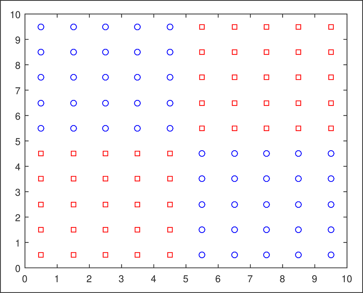
Figure 11
Test region . The intensity function is different in the blue and red subregions, but the user does not know about these subregions. For estimation purposes, the user discretizes into square zones.
7.1.1 Test 1
In this test, the rate function is different on and on , and is periodic with period 2, as follows:
This rate function is represented in Figure 12(a) (for time intervals that start at odd times) and Figure 12(b) (for time intervals that start at even times).
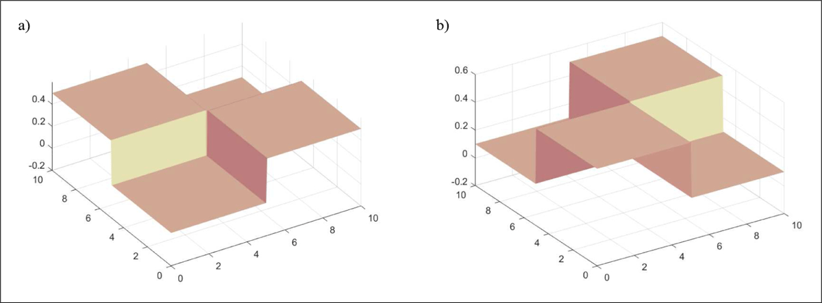
Figure 12
Intensities as a function of location, for time intervals that start at odd times and even times. (a) Time intervals that start at odd times. (b) Time intervals that start at even times.
The user knows the region and that , but does not know about the subregions and that affect the intensity function , and does not know that is periodic with period 2. For estimation purposes, the user discretizes into 100 square zones of unit area each, as shown in Figure 11. Thus indexes two types of zones, but this is not known by the user:
indexes 50 blue zones (with blue circles in their centers in Figure 11); there are 25 blue zones in the bottom right and 25 blue zones in the upper left of the region;
indexes 50 red zones (with red squares in their centers in Figure 11); there are 25 red zones on the bottom left and 25 red zones in the upper right of the region.
Also, for estimation purposes, the user discretizes time into 28 time intervals of length 1 each. Thus, the estimates are denoted with for and . Given arrival data Mi,t,n for , , and , the regularized loss function in (6) is used to estimate . The penalty coefficients are when i,j are neighboring zones, and otherwise, where w will be varied as described later. Two zones are neighbors if their borders share an edge.
We consider two partitions and of time intervals in (6). For partition , the time groups are and . For partition , the time groups are , , , and . For both partitions, penalty coefficients for all groups G (note that all groups have the same cardinality so that it seems reasonable to choose the same weights for different groups). Also, in (17).
For any value of the penalty parameter w, let denote the estimator of produced by (8). Note that when the penalty parameter , then reduces to the empirical estimator of the intensities, which is the mean rate of arrivals in zone i and time interval t. For a range of values of the penalty parameter w, we computed the estimates , and Figure 13 shows the mean (over all zones i and time intervals t) relative error given by
as a function of penalty parameter w, for different values of Ni,t.Figure 13 shows the mean relative errors for the following four estimators: estimator with partition of time intervals and with neighbor-based spatial regularization (legend “4 groups, neighbors” in the figure), estimator with partition of time intervals and without spatial regularization (legend “4 groups, no neighbors” in the figure), estimator with partition of time intervals and with neighbor-based spatial regularization (legend “2 groups, neighbors” in the figure), and estimator with partition of time intervals and without spatial regularization (legend “2 groups, no neighbors” in the figure). Figure 13 presents results for four values of the sample size: , , , and . Figure 13 also shows, for the three larger sample sizes, the mean relative error obtained by choosing the penalty parameter w by cross validation as follows: The data are partitioned into 5 subsets. Then, for each of 5 replications we used one of the data subsets (a different subset for each replication, with 20% of data used for training) to compute for a range of values of w, and we used the remaining data to compute the out-of-sample likelihood value for each value of w. Then we determined the penalty parameter that maximizes the average out-of-sample likelihood value over the 5 replications. Figure 13 shows the mean relative error for the resulting cross validation estimator with partition of time intervals and with neighbor-based spatial regularization using the penalty parameter . Note that the empirical estimator, with , does not depend on the partition of time intervals and the neighbor structure, and therefore is given by all four estimators described above at . Table 1 shows the minimum mean relative errors over different values of penalty parameter w, as well as the values of w that attain the minimum, for each of the four estimators, plus the mean relative errors of the cross validation estimator (using the penalty parameter ) and the empirical estimator (), for each of the four sample sizes considered in Figure 13.
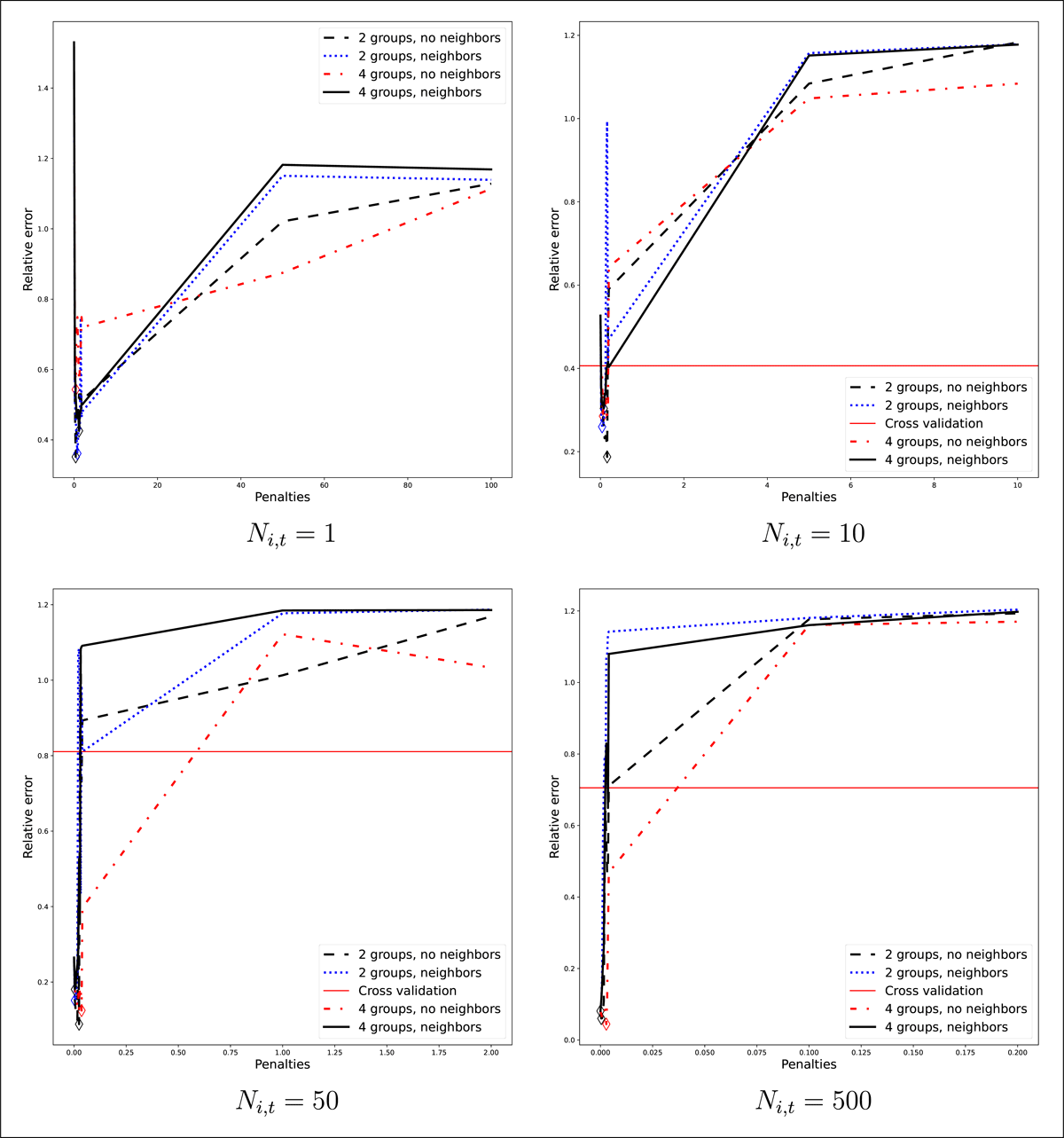
Figure 13
Mean relative estimation errors as a function of the penalty parameter w, for four sample sizes and six estimators (including the empirical estimator at ).
Table 1
The column headings denote the estimators as follows: Reg 1: estimator with partition of time intervals and with neighbor-based spatial regularization; Reg 2: estimator with partition of time intervals and without spatial regularization; Reg 3: estimator with partition of time intervals and with neighbor-based spatial regularization; Reg 4: estimator with partition of time intervals and without spatial regularization; CV: cross validation; Emp: empirical estimator. For each sample size and for each estimator Reg 1, Reg 2, Reg 3, Reg 4, each cell of the table gives two numbers separated by a slash (/): the first number is the minimum mean relative error over different values of penalty parameter w, and the second number is the value of w that attains the minimum. For the cross validation estimator, the first number is the mean relative error using the penalty parameter , and the second number is the value of . For the empirical estimator, the first number is the mean relative error using the penalty parameter .
| SAMPLE SIZE Ni,t | REG 1 | REG 2 | REG 3 | REG 4 | CV | EMP |
|---|---|---|---|---|---|---|
| 1 | 0.47/1.2 | 0.67/2.0 | 0.34/0.6 | 0.51/1.4 | - | 1.539/0 |
| 10 | 0.31/0.06 | 0.30/0.2 | 0.26/0.06 | 0.17/0.2 | 0.42/0.2 | 0.543/0 |
| 50 | 0.18/0.008 | 0.12/0.04 | 0.15/0.004 | 0.08/0.036 | 0.37/0.04 | 0.256/0 |
| 500 | 0.08/0.0 | 0.03/0.004 | 0.08/0.0 | 0.02/0.0028 | 0.26/0.002 | 0.07687/0 |
In Figure 13, note that the vertical and horizontal scales of the sub-figures are different. As expected, the estimation error is decreasing in the sample size Ni,t. Note that the mean relative errors shown in Figure 13, and the values of the penalty parameter w with the smallest mean relative errors (shown with diamonds), were based on using the correct values in the calculations, which are not known by the user. Even when regularization is not based on the correct subregions and partition of time intervals, it can result in better estimates than the empirical estimates (corresponding to ), as long as reasonable values are chosen for w. The results indicate that the improvement of the estimates using regularization is more pronounced when the number of observations is small: for , the estimation error decreases from about 152% (for the empirical estimator) to about 35% for the best regularized estimator, and for , the estimation error decreases from about 52% to about 19%. Therefore, when a small amount of data are available, the regularized estimator results in a smaller estimation error, even if the regularization is not based on the correct model structure, as long as relevant information and reasonable weights are used for the regularization.
Figure 14 shows the true intensities and the estimates obtained with partition of time intervals and with neighbor-based spatial regularization using the cross validation penalty parameters , for , zone , (top left plot), for , zone , (bottom left plot), for , zone , (top right plot), and for , zone , (bottom right plot). It can be seen that if little data are available, then the regularized estimates are closer to the true intensities than the empirical estimates.
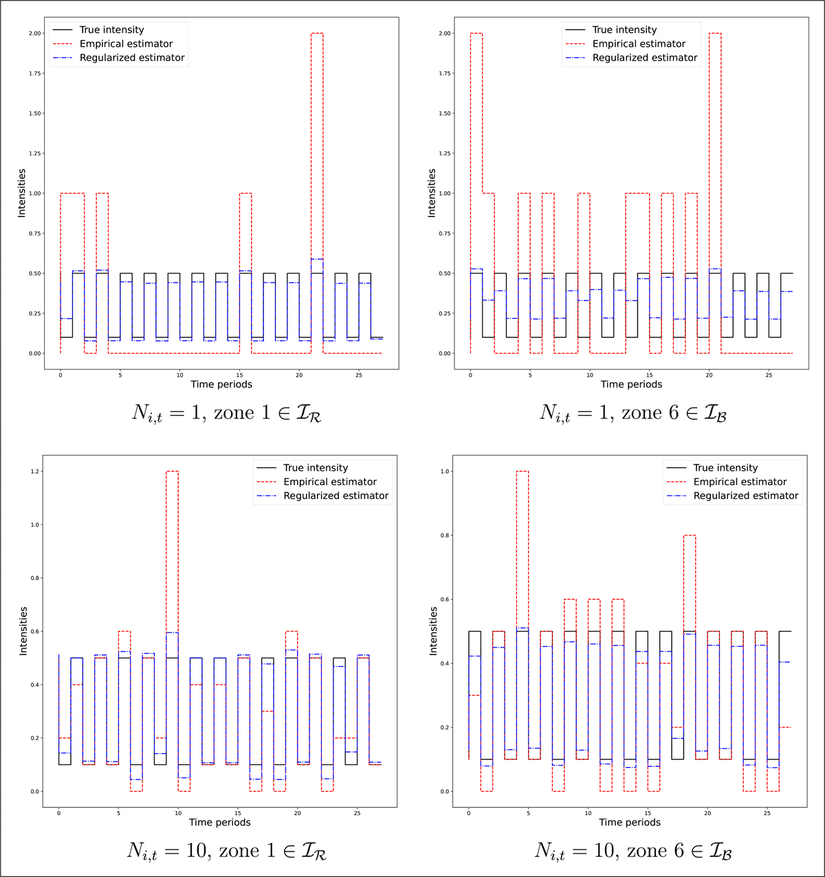
Figure 14
Comparison of true, empirical, and regularized estimates of the Poisson process intensities. True intensities as shown in Figure 12.
7.1.2 Test 2
In this test, we consider the same region and the same subregions and as in Test 1. The intensity function is also periodic, but not piecewise constant, as follows:
This rate function is represented in Figure 15(a) (for time intervals that start at odd times) and Figure 15(b) (for time intervals that start at even times).
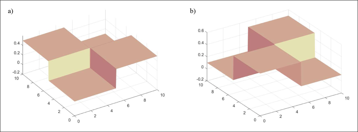
Figure 15
Intensities as a function of location, for time intervals that start at odd times and even times. (a) Time intervals that start at odd times. (b) Time intervals that start at even times.
As in Test 1, the user knows the region and that , but does not know about the subregions and that affect the intensity function , and does not know that is periodic with period 2. For estimation purposes, the user discretizes into 100 square zones of unit area each. The user computes the estimators for each and each , by solving optimization problem (16) using regularization with penalty parameter w and . Each estimator now approximates the rate , where Ri denotes the square of unit area for the zone i. For example, for a zone i with and for , it holds that
where is the centroid of the zone i.
The mean relative error of estimator is now given by
Parameter estimates were computed for a range of values of the penalty parameter w, for the same four estimators as in Test 1: estimator with partition of time intervals and with neighbor-based spatial regularization (legend “4 groups, neighbors” in Figure 16), estimator with partition of time intervals and without spatial regularization (legend “4 groups, no neighbors” in Figure 16), estimator with partition of time intervals and with neighbor-based spatial regularization (legend “2 groups, neighbors” in Figure 16), and estimator with partition of time intervals and without spatial regularization (legend “2 groups, no neighbors” in Figure 16). As before, four values were used for the sample size: , , , and .Figure 16 shows the mean relative error for these four estimators, as well as the estimator with partition of time intervals and with neighbor-based spatial regularization using the penalty parameter chosen with cross validation. As before, the empirical estimator corresponds to . In this test intensities are very different between neighboring zones, and as a result space regularization is not helpful, but if little data are available then time regularization still provides better estimates than the empirical estimator.
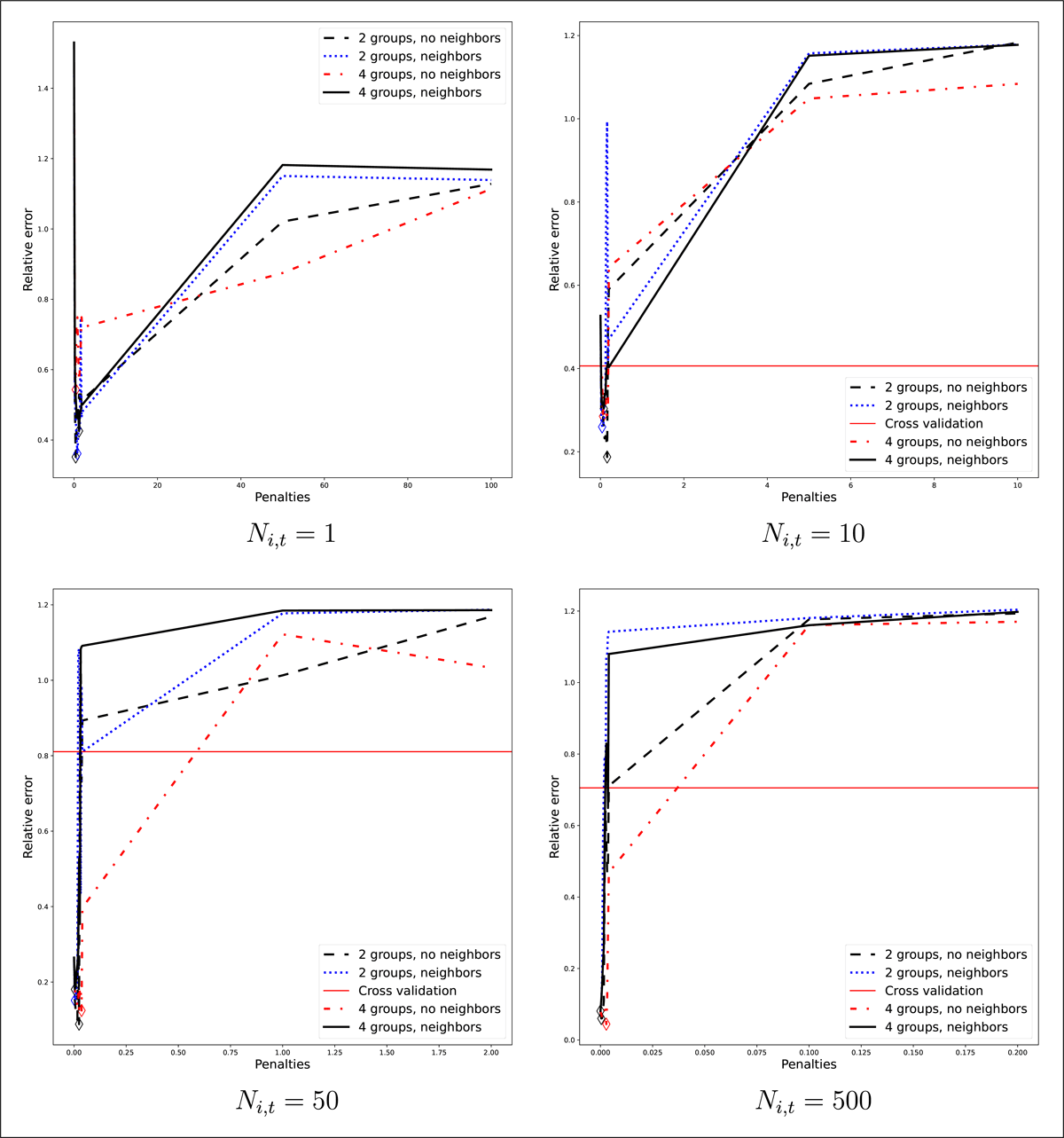
Figure 16
Mean relative errors as a function of the penalty parameter w. Intensities are as shown in Figure 15.
7.2 Quality Control Tests with Artificial Data with Covariates
As in the previous tests, points arrive in and over time according to a periodic non-homogeneous Poisson process. The region is partitioned into two subregions , with and . There is only one type of point, thus , and hence the type notation c is omitted. Each point has three attributes, denoted . For the tests, x(s) was generated as follows. Let , , , be independent random variables uniformly distributed on (0,1). For , let
and for , let
Let and for , and and for . The graph of as a function of the center of the zones is shown in Figure 17.
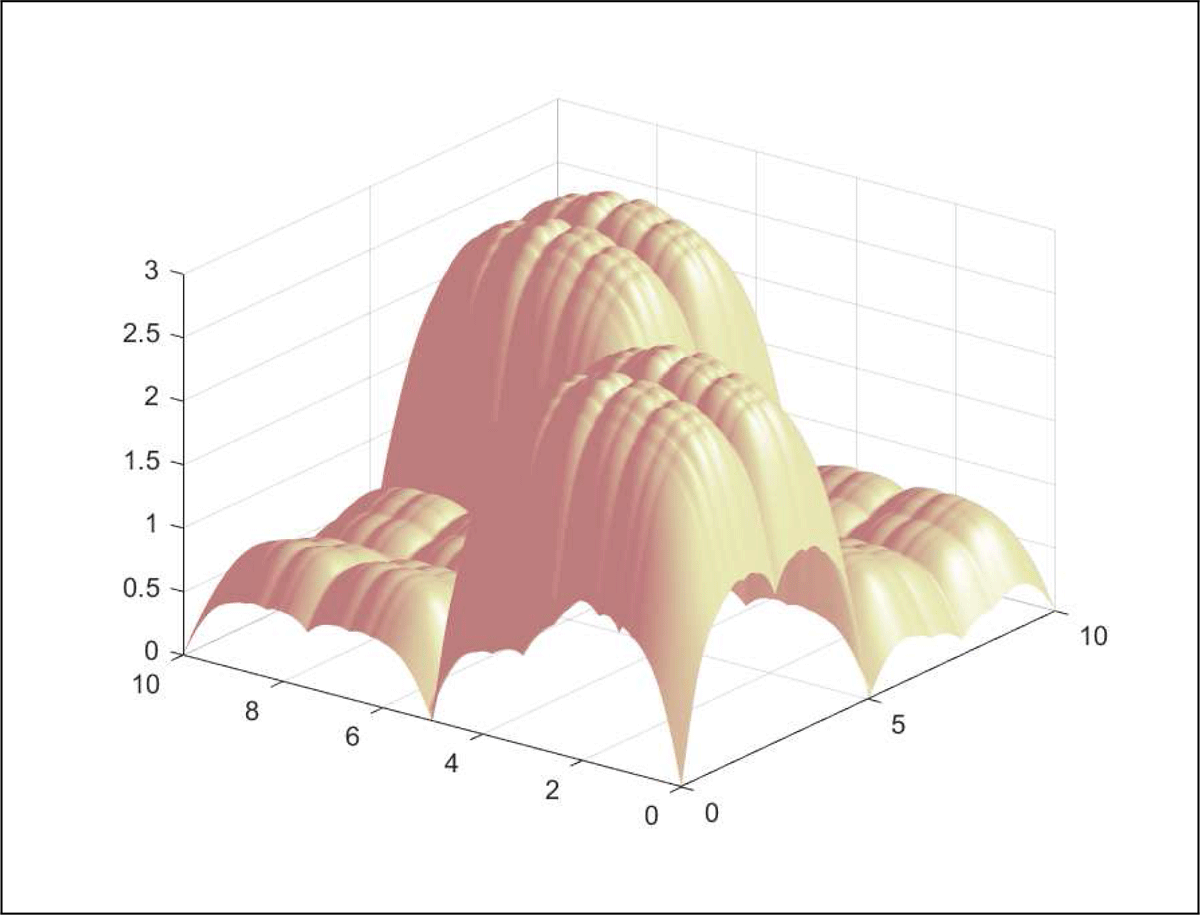
Figure 17
Graph of covariate function x1.
We consider 2 settings, one without a holiday effect, and one with a holiday effect. In both settings, the rate function is periodic with period 2.
7.2.1 Test 3
In the setting without a holiday effect, the rate function is as follows:
where
Thus, if denotes the even-indexed time intervals and denotes the odd-indexed time intervals, and and , then the expected number of arrivals in is given by , where and .
7.2.2 Test 4
In the setting with a holiday effect, the rate function is as follows:
where if t falls in a holiday, and otherwise, and
We consider 2 estimators for each of the 2 settings: one estimator knows and uses aggregated covariate data, and the other estimator does not use covariate data. Below, we describe the 2 estimators in more detail.
7.2.3 Estimators that Use Covariate Data
The user knows the region and that , but does not know that is periodic with period 2. In the setting with a holiday effect, the user knows that there is a holiday effect, but the user distinguishes 8 different holidays and allows them to have different parameters. For estimation purposes, is discretized into 100 square zones of unit area each, as shown in Figure 11. Thus indexes two types of zones, but this is not known by the estimator. For each zone , the user observes only the aggregate value of the covariate xl for the zone. For example, if a zone in is , then the aggregate value of the covariate x1 for the zone is
Therefore, we need to compute integrals of form .
Note that, for , it holds that if
and if
Also note that
Therefore, if , then
and if , then
Also, , and for , and , and for .
As in the previous tests, the user discretizes time into 28 time intervals of length 1 each. The user’s model is the same as the model specified in Example 2.3, with , , , and . Thus, in the setting without a holiday effect, the user’s intensity function given by
estimates , where . Thus, this estimated model has parameters. In the setting with a holiday effect, the user’s intensity function given by
estimates , where if and if , and . Thus, this estimated model has parameters.
7.2.4 Estimators that Do not Use Covariate Data
The user knows the region and that , but does not know the covariate values yi, and does not know that is periodic with period 2. In the setting with a holiday effect, the user knows that there is a holiday effect, but the user distinguishes 8 different holidays and allows them to have different parameters.
The estimators are similar to those in Section 7.1. In the setting without a holiday effect, the user’s intensity function , computed by solving (8) with the penalty parameter w, estimates . In the setting with a holiday effect, the user’s intensity function , computed by solving (8) with the penalty parameter w, estimates .
7.2.5 More quality control tests
Table 2 shows the mean relative errors of regularized estimators with best penalty parameter without covariates from Section 2.1, and the estimator with covariates from Section 2.2 (without regularization). The column “Holiday” indicates whether the intensities used to generate the data are different on holidays or not. For the tests with holidays, in the “Sample size Ni,t” column, the first number is the number of observations for days which are not holidays and the second number is the number of observations for days which are holidays (for instance, for the first experiment with holidays, for periods t which are not on holidays and for periods t which are on holidays). The column “Cov” shows results for the estimator with covariates from Section 2.2. The table also shows results for three regularized estimators without covariates: an estimator that does not use space regularization (column “No Cov 1”), an estimator that uses space regularization with penalizing weights for neighbors of the same color (column “No Cov 2”), and an estimator that uses space regularization with penalizing weights for all neighbors regardless of their color (column “No Cov 3”). For each estimator, the cells in the table show the values of the mean relative error for the estimator and the instance (for the regularized estimators without covariates, the best mean relative error among all considered penalty weights is shown). For this experiment, the best model is the model with covariates.
(2) Availability
Operating system
LASPATED was tested on a Ubuntu Linux 22.04 OS and in a macOS via its Docker container.
Programming language
The discretization features are implemented in Python and is compatible with version Python 3.13. The calibration features are written in C++, compiled and tested with GCC version 11.4. We also provide a Python scripts that performs a basic workflow of the library, generating a space-time discretization and calling the calibration app on the discretized data and a replication script to generate the figures from the Quality Control section.
Additional system requirements
Dependencies
The discretization features depend on the following Python modules: numpy 1.25, pandas 2.0, geopandas 0.12, matplotlib, h3, geovoronoi, rtree, descartes. The LASPATED Python module named laspated is available via pip, that automatically installs these dependencies.
The C++ calibration features depend on Boost 1.74, xtl, xtensor and, optionally, on Gurobi 11.01. The xtl and xtensor are header-only libraries and we provide a copy of them with the source code. Boost is available at https://boost.org and Gurobi is available at https://gurobi.com.
We provide a Docker container that installs all modules and dependencies.
List of contributors
Only the authors of this paper have worked on the development of LASPATED software.
Software location
Archive
Name: Zenodo
Persistent identifier: https://doi.org/10.5281/zenodo.20723233
Licence: Creative Commons Attribution 4.0 International
Publisher: Vincent Guigues
Version published: 1.1.2
Date published: 06/15/2026
Code repository
Name: LASPATED
Persistent identifier: https://github.com/vguigues/LASPATED
Licence: BSD-3-Clause license
Date published: 30/08/2024
Emulation environment
Name: DockerHub
Persistent identifier: https://hub.docker.com/r/victorvhrn/laspated
Licence: BSD-3-Clause license
Date published: 30/08/2024
Language
English
(3) Reuse Potential
The paper describes how the software can be used by both researchers and practitioners, both for data processing functions such as time and space discretizations, and for the calibration of nonhomogeneous Poisson models using spatiotemporal data. The User Manual (26) for the software is available on arXiv. Potential users can also find Youtube videos https://t.ly/O8I3D explaining how to install and use the software with many examples.
Possible extensions of this software include developing and implementing methods to deal with missing data, such as arrivals with missing location data, and methods of adaptive discretization (data-dependent discretization).
Users that encounter an issue can post it online on the github page of the project as a github issue.
Author Contributions
All authors participated equally to the development of models and implementation of the software.